Exercises

Exercise 73: Understand why Newton's method can fail

The purpose of this exercise is to understand when Newton's method works and fails. To this end, solve $ \tanh x=0 $ by Newton's method and study the intermediate details of the algorithm. Start with $ x_0=1.08 $. Plot the tangent in each iteration of Newton's method. Then repeat the calculations and the plotting when $ x_0=1.09 $. Explain what you observe.

Solution.

The program may be written as:

from numpy import tanh, linspace
import matplotlib.pyplot as plt

def Newton_failure(f, dfdx, x, eps):
    f_value = f(x)
    iteration_counter = 0
    while abs(f_value) > eps and iteration_counter < 100:
        try:
            print 'Current x value: ', x
            plot_line(f, x, f_value, dfdx(x))
            raw_input('...press enter to continue')
            x = x - float(f_value)/dfdx(x)
        except ZeroDivisionError:
            print "Error! - derivative zero for x = ", x
            sys.exit(1)     # Abort with error
            
        f_value = f(x)
        iteration_counter += 1

    # Here, either a solution is found, or too many iterations
    if abs(f_value) > eps:
        iteration_counter = -1
    return x, iteration_counter

def f(x):
    return tanh(x)
    
def dfdx(x):
    return 1 - tanh(x)**2
    
def plot_line(f, xn, f_xn, slope):
    # Plot both f(x) and the tangent
    x_f = linspace(-2,2,100)
    y_f = f(x_f)
    x_t = linspace(xn-2,xn+2,10)
    y_t = slope*x_t + (f_xn - slope*xn)  # Straight line: ax + b
    plt.figure() 
    plt.plot(x_t, y_t, 'r-', x_f, y_f, 'b-');    plt.grid('on')
    plt.xlabel('x');    plt.ylabel('f(x)')
    plt.show()

def application():
    solution, no_iterations = \
                      Newton_failure(f, dfdx, x=1.09, eps=0.001)
    
    if no_iterations > 0:    # Solution found
        print "Number of function calls: %d" % (1 + 2*no_iterations)    
        print "A solution is: %f" % (solution)
    else:
        print "Solution not found!"

if __name__ == '__main__':
    application()

Running the program with x set to $ 1.08 $ produces a series of plots (and prints) showing the graph and the tangent for the present value of x. There are quite many plots, so we do not show them here. However, the tangent line "jumps" around a few times before it settles. In the final plot the tangent line goes through the solution at $ x = 0 $. The final printout brings the information:

Number of function calls: 13
A solution is: 0.000024

When we run the program anew, this time with x set to $ 1.09 $, we get another series of plots (and prints), but this time the tangent moves away from the (known) solution. The final printout we get states that:

Number of function calls: 19
A solution is: nan

Here, nan stands for "not a number", meaning that we got no solution value for x. That is, Newton's method diverged.

Filename: Newton_failure.*.

Exercise 74: See if the secant method fails

Does the secant method behave better than Newton's method in the problem described in Exercise 73: Understand why Newton's method can fail? Try the initial guesses

$ x_0=1.08 $ and $ x_1=1.09 $
$ x_0=1.09 $ and $ x_1=1.1 $
$ x_0=1 $ and $ x_1=2.3 $
$ x_0=1 $ and $ x_1=2.4 $

Solution.

The program may be written as:

import sys
from Newton_failure import f, dfdx, plot_line

def secant_failure(f, x0, x1, eps):
    f_x0 = f(x0)
    f_x1 = f(x1)
    iteration_counter = 0

    while abs(f_x1) > eps and iteration_counter < 100:
        try:
            print 'Current x value: ', x1
            denominator = float(f_x1 - f_x0)/(x1 - x0)
            plot_line(f, x1, f_x1, denominator)
            raw_input('...press enter to continue')
            x = x1 - float(f_x1)/denominator
        except ZeroDivisionError:
            print "Error! - denominator zero for x = ", x
            sys.exit(1)     # Abort with error
        x0 = x1;
        x1 = x
        f_x0 = f_x1;
        f_x1 = f(x1)
        iteration_counter += 1

    # Here, either a solution is found, or too many iterations
    if abs(f_x1) > eps:
        iteration_counter = -1
    return x, iteration_counter

#x0 = 1.08;   x1 = 1.09
#x0 = 1.09;   x1 = 1.1
#x0 = 1.0;   x1 = 2.3
x0 = 1.0;   x1 = 2.4
error_limit = 1e-6

solution, no_iterations = secant_failure(f, x0, x1, eps=1.0e-6)

if no_iterations > 0:    # Solution found
    print "Number of function calls: %d" % (2 + no_iterations)
    print "A solution is: %f" % (solution)
else:
    print "Solution not found!"

The script converges with the three first-mentioned alternatives for $ x_0 $ and $ x_1 $. With the final set of parameter values, the method diverges with a printout:

Error! - denominator zero for x = 360.600893792

and a few more lines stating that an exception error has occurred.

Filename: secant_failure.*.

Exercise 75: Understand why the bisection method cannot fail

Solve the same problem as in Exercise 73: Understand why Newton's method can fail, using the bisection method, but let the initial interval be $ [-5,3] $. Report how the interval containing the solution evolves during the iterations.

Solution.

The code may be written as:

from math import tanh

def bisection_nonfailure(f, x_L, x_R, eps, return_x_list=False):
    f_L = f(x_L)
    if f_L*f(x_R) > 0:
        print "Error! Function dow not have opposite \
                  signs at interval endpoints!"
        sys.exit(1)
    x_M = float(x_L + x_R)/2.0
    f_M = f(x_M)
    iteration_counter = 1
    if return_x_list:
        x_list = []
    
    while abs(f_M) > eps:
        if f_L*f_M > 0:   # i.e. same sign
            x_L = x_M
            f_L = f_M
        else:
            x_R = x_M
        print 'interval: [%f, %f]' % (x_L, x_R) # print new interval
        x_M = float(x_L + x_R)/2
        f_M = f(x_M)
        iteration_counter += 1
        if return_x_list:
            x_list, append(x_M)
    if return_x_list:
        return x_list, iteration_counter
    else:
        return x_M, iteration_counter

def f(x):
    return tanh(x)

a = -5;  b = 3

solution, no_iterations = bisection_nonfailure(f, a, b, eps=1.0e-6)

print "Number of function calls: %d" % (1 + 2*no_iterations)
print "A solution is: %f" % (solution)

Running the program produces the following printout:

interval: [-1.000000, 3.000000]
interval: [-1.000000, 1.000000]
Number of function calls: 7
A solution is: 0.000000

Filename: bisection_nonfailure.*.

Exercise 76: Combine the bisection method with Newton's method

An attractive idea is to combine the reliability of the bisection method with the speed of Newton's method. Such a combination is implemented by running the bisection method until we have a narrow interval, and then switch to Newton's method for speed.

Write a function that implements this idea. Start with an interval $ [a,b] $ and switch to Newton's method when the current interval in the bisection method is a fraction $ s $ of the initial interval (i.e., when the interval has length $ s(b-a) $). Potential divergence of Newton's method is still an issue, so if the approximate root jumps out of the narrowed interval (where the solution is known to lie), one can switch back to the bisection method. The value of $ s $ must be given as an argument to the function, but it may have a default value of 0.1.

Try the new method on $ \tanh(x)=0 $ with an initial interval $ [-10,15] $.

Solution.

The code may be written as:

from numpy import tanh
from Newtons_method import Newton

def bisection_Newton(f, dfdx, x_L, x_R, eps, s=0.1):
    f_L = f(x_L)
    if f_L*f(x_R) > 0:
        print "Error! Function does not have opposite \
                  signs at interval endpoints!"
        sys.exit(1)
    x_M = float(x_L + x_R)/2.0
    f_M = f(x_M)
    iteration_counter = 1
    interval_Newton = s*(x_R - x_L)    # Limit for swith to Newton
    
    while (x_R - x_L) > interval_Newton:
        if f_L*f_M > 0:   # i.e. same sign
            x_L = x_M
            f_L = f_M
        else:
            x_R = x_M
        x_M = float(x_L + x_R)/2
        f_M = f(x_M)
        iteration_counter += 1
    solution, no_iterations = Newton(f, dfdx, x_M, eps)
    return solution, (iteration_counter + no_iterations)

def f(x):
    return tanh(x)

def dfdx(x):
    return 1 - tanh(x)**2

eps = 1e-6
a = -10;   b = 15

solution, no_iterations = \
                     bisection_Newton(f, dfdx, a, b, eps)
print "A solution x = %f was reached in %d iterations" % \
                                   (solution,no_iterations)

Running the program produces the following printout:

A solution x = 0.000000 was reached in 7 iterations

Filename: bisection_Newton.py.

Exercise 77: Write a test function for Newton's method

The purpose of this function is to verify the implementation of Newton's method in the Newton function in the file nonlinear_solvers.py. Construct an algebraic equation and perform two iterations of Newton's method by hand or with the aid of SymPy. Find the corresponding size of $ |f(x)| $ and use this as value for eps when calling Newton. The function should then also perform two iterations and return the same approximation to the root as you calculated manually. Implement this idea for a unit test as a test function test_Newton().

Solution.

Here is the complete module with the test function. We use SymPy to do the manual calculations.

from nonlinear_solvers import Newton

def test_Newton():
    # Construct test problem and run two iterations
    import sympy as sp
    x = sp.symbols('x')
    f = sp.cos(x) + sp.sin(x)  # equation f(x)=0
    dfdx = sp.diff(f, x)
    x0 = 2                     # initial guess
    # Run two iterations with Newton's method
    x1 = x0 - f.subs(x, x0)/dfdx.subs(x, x0)
    x_expected = [x1.evalf()]  # convert to float
    x2 = x1 - f.subs(x, x1)/dfdx.subs(x, x1)
    x_expected.append(x2.evalf())
    f = sp.lambdify([x], f)
    eps = f(x_expected[-1])  # this eps gives two iterations

    dfdx = sp.lambdify([x], dfdx)
    x_computed, it_counter = Newton(f, dfdx, x0, eps, True)
    assert it_counter == 2
    tol = 1E-15
    assert abs(x_computed[0] - x_expected[0]) < tol
    assert abs(x_computed[1] - x_expected[1]) < tol

if __name__ == '__main__':
    test_Newton()

Filename: test_Newton.py.

Exercise 78: Solve nonlinear equation for a vibrating beam

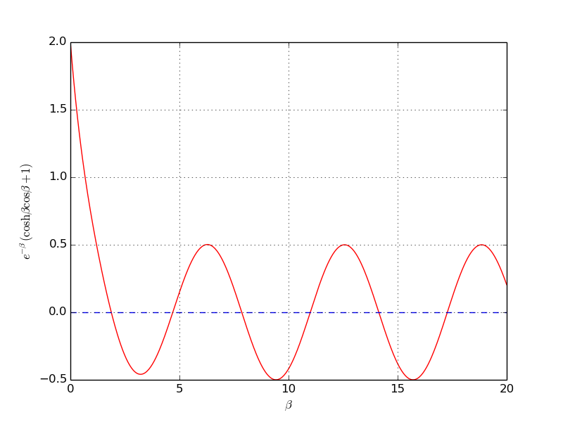
An important engineering problem that arises in a lot of applications is the vibrations of a clamped beam where the other end is free. This problem can be analyzed analytically, but the calculations boil down to solving the following nonlinear algebraic equation: $$ \cosh\beta \cos\beta = -1,$$ where $ \beta $ is related to important beam parameters through $$ \beta^4 = \omega^2 \frac{\varrho A}{EI},$$ where $ \varrho $ is the density of the beam, $ A $ is the area of the cross section, $ E $ is Young's modulus, and $ I $ is the moment of the inertia of the cross section. The most important parameter of interest is $ \omega $, which is the frequency of the beam. We want to compute the frequencies of a vibrating steel beam with a rectangular cross section having width $ b=25 $ mm and height $ h=8 $ mm. The density of steel is $ 7850 \mbox{ kg/m}^3 $, and $ E= 2\cdot 10^{11} $ Pa. The moment of inertia of a rectangular cross section is $ I=bh^3/12 $.

a) Plot the equation to be solved so that one can inspect where the zero crossings occur.

Hint.

When writing the equation as $ f(\beta)=0 $, the $ f $ function increases its amplitude dramatically with $ \beta $. It is therefore wise to look at an equation with damped amplitude, $ g(\beta) = e^{-\beta}f(\beta) = 0 $. Plot $ g $ instead.

Solution.

b) Compute the first three frequencies.

Solution.

Here is a complete program, using the Bisection method for root finding, based on intervals found from the plot above.

from numpy import *
from matplotlib.pyplot import *

def f(beta):
    return cosh(beta)*cos(beta) + 1

def damped(beta):
    """Damp the amplitude of f. It grows like cosh, i.e. exp."""
    return exp(-beta)*f(beta)

def plot_f():
    beta = linspace(0, 20, 501)
    #y = f(x)
    y = damped(beta)
    plot(beta, y, 'r', [beta[0], beta[-1]], [0, 0], 'b--')
    grid('on')
    xlabel(r'$\beta$')
    ylabel(r'$e^{-\beta}(\cosh\beta\cos\beta +1)$')
    savefig('tmp1.png'); savefig('tmp1.pdf')
    show()

plot_f()

from nonlinear_solvers import bisection
# Set up suitable intervals
intervals = [[1, 3], [4, 6], [7, 9]]
betas = []  # roots
for beta_L, beta_R in intervals:
    beta, it = bisection(f, beta_L, beta_R, eps=1E-6)
    betas.append(beta)
    print f(beta)
print betas

# Find corresponding frequencies

def omega(beta, rho, A, E, I):
    return sqrt(beta**4/(rho*A/(E*I)))

rho = 7850  # kg/m^3
E = 1.0E+11 # Pa
b = 0.025   # m
h = 0.008   # m
A = b*h
I = b*h**3/12

for beta in betas:
    print omega(beta, rho, A, E, I)

The output of $ \beta $ reads $ 1.875 $, $ 4.494 $, $ 7.855 $, and corresponding $ \omega $ values are $ 29 $, $ 182 $, and $ 509 $ Hz.

Filename: beam_vib.py.