The composite trapezoidal rule

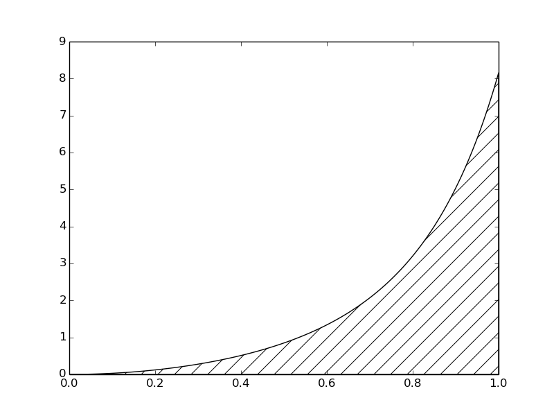
The integral \( \int_a^b f(x)dx \) may be interpreted as the area between the \( x \) axis and the graph \( y=f(x) \) of the integrand. Figure 7 illustrates this area for the choice (3.7). Computing the integral \( \int_0^1f(t)dt \) amounts to computing the area of the hatched region.

If we replace the true graph in Figure 7 by a set of straight line segments, we may view the area rather as composed of trapezoids, the areas of which are easy to compute. This is illustrated in Figure 8, where 4 straight line segments give rise to 4 trapezoids, covering the time intervals \( [0,0.2) \), \( [0.2,0.6) \), \( [0.6,0.8) \) and \( [0.8,1.0] \). Note that we have taken the opportunity here to demonstrate the computations with time intervals that differ in size.

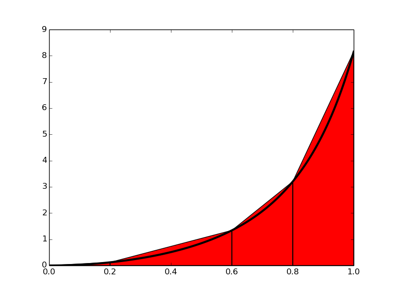
The areas of the 4 trapezoids shown in Figure 8 now constitute our approximation to the integral (3.7): $$ \begin{align} \int_0^1 v(t)dt &\approx h_1 (\frac{v(0)+v(0.2)}{2}) + h_2 (\frac{v(0.2)+v(0.6)}{2}) \nonumber \\ &+ h_3 (\frac{v(0.6)+v(0.8)}{2}) + h_4 (\frac{v(0.8)+v(1.0)}{2}), \tag{3.9} \end{align} $$ where $$ \begin{align} h_1 &= (0.2 - 0.0), \tag{3.10} \\ h_2 &= (0.6 - 0.2), \tag{3.11} \\ h_3 &= (0.8 - 0.6), \tag{3.12} \\ h_4 &= (1.0 - 0.8)\thinspace \tag{3.13} \end{align} $$ With \( v(t) = 3t^{2}e^{t^3} \), each term in (3.9) is readily computed and our approximate computation gives $$ \begin{equation} \int_0^1 v(t)dt \approx 1.895\thinspace . \tag{3.14} \end{equation} $$ Compared to the true answer of \( 1.718 \), this is off by about 10%. However, note that we used just 4 trapezoids to approximate the area. With more trapezoids, the approximation would have become better, since the straight line segments in the upper trapezoid side then would follow the graph more closely. Doing another hand calculation with more trapezoids is not too tempting for a lazy human, though, but it is a perfect job for a computer! Let us therefore derive the expressions for approximating the integral by an arbitrary number of trapezoids.

The general formula

For a given function \( f(x) \), we want to approximate the integral \( \int_a^bf(x)dx \) by \( n \) trapezoids (of equal width). We start out with (3.5) and approximate each integral on the right hand side with a single trapezoid. In detail, $$ \begin{align} \int_a^b f(x)\,dx &= \int_{x_0}^{x_1} f(x) dx + \int_{x_1}^{x_2} f(x) dx + \ldots + \int_{x_{n-1}}^{x_n} f(x) dx, \nonumber \\ &\approx h \frac{f(x_0) + f(x_1)}{2} + h \frac{f(x_1) + f(x_2)}{2} + \ldots + \nonumber \\ &\quad h \frac{f(x_{n-1}) + f(x_n)}{2} \tag{3.15} \end{align} $$ By simplifying the right hand side of (3.15) we get $$ \begin{equation} \int_a^b f(x)\,dx \approx \\ \frac{h}{2}\left[f(x_0) + 2 f(x_1) + 2 f(x_2) + \ldots + 2 f(x_{n-1}) + f(x_n)\right] \tag{3.16} \end{equation} $$ which is more compactly written as $$ \begin{equation} \int_a^b f(x)\,dx \approx h \left[\frac{1}{2}f(x_0) + \sum_{i=1}^{n-1}f(x_i) + \frac{1}{2}f(x_n) \right] \thinspace . \tag{3.17} \end{equation} $$

Implementation

Specific or general implementation?

Suppose our primary goal was to compute the specific integral \( \int_0^1 v(t)dt \) with \( v(t)=3t^2e^{t^3} \). First we played around with a simple hand calculation to see what the method was about, before we (as one often does in mathematics) developed a general formula (3.17) for the general or "abstract" integral \( \int_a^bf(x)dx \). To solve our specific problem \( \int_0^1 v(t)dt \) we must then apply the general formula (3.17) to the given data (function and integral limits) in our problem. Although simple in principle, the practical steps are confusing for many because the notation in the abstract problem in (3.17) differs from the notation in our special problem. Clearly, the \( f \), \( x \), and \( h \) in (3.17) correspond to \( v \), \( t \), and perhaps \( \Delta t \) for the trapezoid width in our special problem.

The first alternative in the box above sounds less abstract and therefore more attractive to many. Nevertheless, as we hope will be evident from the examples, the second alternative is actually the simplest and most reliable from both a mathematical and programming point of view. These authors will claim that the second alternative is the essence of the power of mathematics, while the first alternative is the source of much confusion about mathematics!

Implementation with functions

For the integral \( \int_a^bf(x)dx \) computed by the formula (3.17) we want the corresponding Python function trapezoid to take any \( f \), \( a \), \( b \), and \( n \) as input and return the approximation to the integral.

We write a Python function trapezoidal in a file trapezoidal.py as close as possible to the formula (3.17), making sure variable names correspond to the mathematical notation:

def trapezoidal(f, a, b, n):
    h = float(b-a)/n
    result = 0.5*f(a) + 0.5*f(b)
    for i in range(1, n):
        result += f(a + i*h)
    result *= h
    return result

Solving our specific problem in a session

Just having the trapezoidal function as the only content of a file trapezoidal.py automatically makes that file a module that we can import and test in an interactive session:

>>> from trapezoidal import trapezoidal
>>> from math import exp
>>> v = lambda t: 3*(t**2)*exp(t**3)
>>> n = 4
>>> numerical = trapezoidal(v, 0, 1, n)
>>> numerical
1.9227167504675762

Let us compute the exact expression and the error in the approximation:

>>> V = lambda t: exp(t**3)
>>> exact = V(1) - V(0)
>>> exact - numerical
-0.20443492200853108

Is this error convincing? We can try a larger \( n \):

>>> numerical = trapezoidal(v, 0, 1, n=400)
>>> exact - numerical
-2.1236490512777095e-05

Fortunately, many more trapezoids give a much smaller error.

Solving our specific problem in a program

Instead of computing our special problem in an interactive session, we can do it in a program. As always, a chunk of code doing a particular thing is best isolated as a function even if we do not see any future reason to call the function several times and even if we have no need for arguments to parameterize what goes on inside the function. In the present case, we just put the statements we otherwise would have put in a main program, inside a function:

def application():
    from math import exp
    v = lambda t: 3*(t**2)*exp(t**3)
    n = input('n: ')
    numerical = trapezoidal(v, 0, 1, n)

    # Compare with exact result
    V = lambda t: exp(t**3)
    exact = V(1) - V(0)
    error = exact - numerical
    print 'n=%d: %.16f, error: %g' % (n, numerical, error)

Now we compute our special problem by calling application() as the only statement in the main program. Both the trapezoidal and application functions reside in the file trapezoidal.py, which can be run as

Terminal> python trapezoidal.py
n: 4
n=4: 1.9227167504675762, error: -0.204435

Making a module

When we have the different pieces of our program as a collection of functions, it is very straightforward to create a module that can be imported in other programs. That is, having our code as a module, means that the trapezoidal function can easily be reused by other programs to solve other problems. The requirements of a module are simple: put everything inside functions and let function calls in the main program be in the so-called test block:

if __name__ == '__main__':
    application()

The if test is true if the module file, trapezoidal.py, is run as a program and false if the module is imported in another program. Consequently, when we do an import from trapezoidal import trapezoidal in some file, the test fails and application() is not called, i.e., our special problem is not solved and will not print anything on the screen. On the other hand, if we run trapezoidal.py in the terminal window, the test condition is positive, application() is called, and we get output in the window:

Terminal> python trapezoidal.py
n: 400
n=400: 1.7183030649495579, error: -2.12365e-05

Alternative flat special-purpose implementation

Let us illustrate the implementation implied by alternative 1 in the Programmer's dilemma box in the section Implementation. That is, we make a special-purpose code where we adapt the general formula (3.17) to the specific problem \( \int_0^1 3t^2e^{t^3}dt \).

Basically, we use a for loop to compute the sum. Each term with \( f(x) \) in the formula (3.17) is replaced by \( 3t^2e^{t^3} \), \( x \) by \( t \), and \( h \) by \( \Delta t \) 1. A first try at writing a plain, flat program doing the special calculation is

from math import exp

a = 0.0;  b = 1.0
n = input('n: ')
dt = float(b - a)/n

# Integral by the trapezoidal method
numerical = 0.5*3*(a**2)*exp(a**3) + 0.5*3*(b**2)*exp(b**3)
for i in range(1, n):
    numerical += 3*((a + i*dt)**2)*exp((a + i*dt)**3)
numerical *= dt

exact_value = exp(1**3) - exp(0**3)
error = abs(exact_value - numerical)
rel_error = (error/exact_value)*100
print 'n=%d: %.16f, error: %g' % (n, numerical, error)

1: Replacing \( h \) by \( \Delta t \) is not strictly required as many use \( h \) as interval also along the time axis. Nevertheless, \( \Delta t \) is an even more popular notation for a small time interval, so we adopt that common notation.

The problem with the above code is at least three-fold:

1. We need to reformulate (3.17) for our special problem with a different notation.
2. The integrand \( 3t^2e^{t^3} \) is inserted many times in the code, which quickly leads to errors.
3. A lot of edits are necessary to use the code to compute a different integral - these edits are likely to introduce errors.

from math import exp

v = lambda t: 3*(t**2)*exp(t**3)  # Function to be integrated
a = 0.0;  b = 1.0
n = input('n: ')
dt = float(b - a)/n

# Integral by the trapezoidal method
numerical = 0.5*v(a) + 0.5*v(b)
for i in range(1, n):
    numerical += v(a + i*dt)
numerical *= dt

F = lambda t: exp(t**3)
exact_value = F(b) - F(a)
error = abs(exact_value - numerical)
rel_error = (error/exact_value)*100
print 'n=%d: %.16f, error: %g' % (n, numerical, error)

Unfortunately, the two other problems remain and they are fundamental.

Suppose you want to compute another integral, say \( \int_{-1}^{1.1}e^{-x^2}dx \). How much do we need to change in the previous code to compute the new integral? Not so much:

• the formula for v must be replaced by a new formula
• the limits a and b
• the anti-derivative \( V \) is not easily known 2 and can be omitted, and therefore we cannot write out the error
• the notation should be changed to be aligned with the new problem, i.e., t and dt changed to x and h

2: You cannot integrate \( e^{-x^2} \) by hand, but this particular integral is appearing so often in so many contexts that the integral is a special function, called the Error function and written \( \mbox{erf}(x) \). In a code, you can call erf(x). The erf function is found in the math module.

These changes are straightforward to implement, but they are scattered around in the program, a fact that requires us to be very careful so we do not introduce new programming errors while we modify the code. It is also very easy to forget to make a required change.

With the previous code in trapezoidal.py, we can compute the new integral \( \int_{-1}^{1.1}e^{-x^2}dx \) without touching the mathematical algorithm. In an interactive session (or in a program) we can just do

>>> from trapezoidal import trapezoidal
>>> from math import exp
>>> trapezoidal(lambda x: exp(-x**2), -1, 1.1, 400)
1.5268823686123285

When you now look back at the two solutions, the flat special-purpose program and the function-based program with the general-purpose function trapezoidal, you hopefully realize that implementing a general mathematical algorithm in a general function requires somewhat more abstract thinking, but the resulting code can be used over and over again. Essentially, if you apply the flat special-purpose style, you have to retest the implementation of the algorithm after every change of the program.

The present integral problems result in short code. In more challenging engineering problems the code quickly grows to hundreds and thousands of line. Without abstractions in terms of general algorithms in general reusable functions, the complexity of the program grows so fast that it will be extremely difficult to make sure that the program works properly.

Another advantage of packaging mathematical algorithms in functions is that a function can be reused by anyone to solve a problem by just calling the function with a proper set of arguments. Understanding the function's inner details is not necessary to compute a new integral. Similarly, you can find libraries of functions on the Internet and use these functions to solve your problems without specific knowledge of every mathematical detail in the functions.

This desirable feature has its downside, of course: the user of a function may misuse it, and the function may contain programming errors and lead to wrong answers. Testing the output of downloaded functions is therefore extremely important before relying on the results.

• ← Prev
• Next →