More basic concepts

So far we have seen a few basic examples on how to apply Python programming to solve mathematical problems. Before we can go on with other and more realistic examples, we need to briefly treat some topics that will be frequently required in later chapters. These topics include computer science concepts like variables, objects, error messages, and warnings; more numerical concepts like rounding errors, arithmetic operator precedence, and integer division; in addition to more Python functionality when working with arrays, plotting, and printing.

Using Python interactively

Python can also be used interactively. That is, we do not first write a program in a file and execute it, but we give statements and expressions to what is known as a Python shell. We recommend to use IPython as shell (because it is superior to alternative Python shells). With Spyder, Ipython is available at startup, appearing as the lower right window. Following the IPython prompt In [1]: (a prompt means a "ready sign", i.e. the program allows you to enter a command, and different programs often have different looking prompts), you may do calculations:

In  [1]: 2+2
Out [1]: 4

In  [2]: 2*3
Out [2]: 6

In  [3]: 10/2
Out [3]: 5

In  [4]: 2**3
Out [4]: 8

The response from IPython is preceded by Out [q]:, where q equals p when the response is to input "number" p.

Note that, as in a program, you may have to use import before using pi or functions like sin, cos, etc. That is, at the prompt, do the command from math import * before you use pi or sin, etc. Importing other modules than math may be relevant, depending on what your aim is with the computations.

You may also define variables and use formulas interactively as

In [1]: v0 = 5

In [2]: g = 9.81

In [3]: t = 0.6

In [4]: y = v0*t - 0.5*g*t**2

In [5]: print y
------> print(y)
1.2342

Sometimes you would like to repeat a command you have given earlier, or perhaps give a command that is almost the same as an earlier one. Then you can use the up-arrow key. Pressing this one time gives you the previous command, pressing two times gives you the command before that, and so on. With the down-arrow key you can go forward again. When you have the relevant command at the prompt, you may edit it before pressing enter (which lets Python read it and take action).

Arithmetics, parentheses and rounding errors

When the arithmetic operators +, -, *, / and ** appear in an expression, Python gives them a certain precedence. Python interprets the expression from left to right, taking one term (part of expression between two successive + or -) at a time. Within each term, ** is done before * and /. Consider the expression x = 1*5**2 + 10*3 - 1.0/4. There are three terms here and interpreting this, Python starts from the left. In the first term, 1*5**2, it first does 5**2 which equals 25. This is then multiplied by 1 to give 25 again. The second term is 10*3, i.e., 30. So the first two terms add up to 55. The last term gives 0.25, so the final result is 54.75 which becomes the value of x.

Note that parentheses are often very important to group parts of expressions together in the intended way. Let us say x = 4 and that you want to divide 1.0 by x + 1. We know the answer is 0.2, but the way we present the task to Python is critical, as shown by the following example.

In [1]: x = 4

In  [2]: 1.0/x+1
Out [2]: 1.25

In  [3]: 1.0/(x+1)
Out [3]: 0.20000000000000001

In the first try, we see that 1.0 is divided by x (i.e., 4), giving 0.25, which is then added to 1. Python did not understand that our complete denominator was x+1. In our second try, we used parentheses to "group" the denominator, and we got what we wanted. That is, almost what we wanted! Since most numbers can be represented only approximately on the computer, this gives rise to what is called rounding errors. We should have got 0.2 as our answer, but the inexact number representation gave a small error. Usually, such errors are so small compared to the other numbers of the calculation, that we do not need to bother with them. Still, keep it in mind, since you will encounter this issue from time to time. More details regarding number representations on a computer is given in the section Finite precision of floating-point numbers.

Variables and objects

Variables in Python will be of a certain type. If you have an integer, say you have written x = 2 in some Python program, then x becomes an integer variable, i.e., a variable of type int. Similarly, with the statement x = 2.0, x becomes a float variable (the word float is just computer language for a real number). In any case, Python thinks of x as an object, of type int or float. Another common type of variable is str, i.e. a string, needed when you want to store text. When Python interprets x = "This is a string", it stores the text (in between the quotes) in the variable x. This variable is then an object of type str. You may convert between variable types if it makes sense. If, e.g., x is an int object, writing y = float(x) will make y a floating point representation of x. Similarly, you may write int(x) to produce an int if x is originally of type float. Type conversion may also occur automatically, as shown just below.

Names of variables should be chosen so that they are descriptive. When computing a mathematical quantity that has some standard symbol, e.g. \( \alpha \), this should be reflected in the name by letting the word alpha be part of the name for the corresponding variable in the program. If you, e.g., have a variable for counting the number of sheep, then one appropriate name could be no_of_sheep. Such naming makes it much easier for a human to understand the written code. Variable names may also contain any digit from 0 to 9, or underscores, but can not start with a digit. Letters may be lower or upper case, which to Python is different. Note that certain names in Python are reserved, meaning that you can not use these as names for variables. Some examples are for, while, if, else, global, return and elif. If you accidentally use a reserved word as a variable name you get an error message.

We have seen that, e.g., x = 2 will assign the value 2 to the variable x. But how do we write it if we want to increase x by 4? We may write an assignment like x = x + 4, or (giving a faster computation) x += 4. Now Python interprets this as: take whatever value that is in x, add 4, and let the result become the new value of x. In other words, the old value of x is used on the right hand side of =, no matter how messy the expression might be, and the result becomes the new value of x. In a similar way, x -= 4 reduces the value of x by 4, x *= 4 multiplies x by 4, and x /= 4 divides x by 4, updating the value of x accordingly.

What if x = 2, i.e., an object of type int, and we add 4.0, i.e., a float? Then automatic type conversion takes place, and the new x will have the value 6.0, i.e., an object of type float as seen here,

In  [1]: x = 2

In  [2]: x = x + 4.0

In  [3]: x
Out [3]: 6.0

Note that Python programmers, and Python (in printouts), often write, e.g., \( 2. \) which by definition is the integer \( 2 \) represented as a float.

Integer division

Another issue that is important to be aware of is integer division. Let us look at a small example, assuming we want to divide one by four.

In  [1]: 1/4
Out [1]: 0

In  [2]: 1.0/4
Out [2]: 0.25

We see two alternative ways of writing it, but only the last way of writing it gave the correct (i.e., expected) result! Why?

With Python version 2, the first alternative gives what is called integer division, i.e., all decimals in the answer are disregarded, so the result is rounded down to the nearest integer. To avoid it, we may introduce an explicit decimal point in either the numerator, the denominator, or in both. If you are new to programming, this is certainly strange behavior. However, you will find the same feature in many programming languages, not only Python, but actually all languages with significant inheritance from C. If your numerator or denominator is a variable, say you have 1/x, you may write 1/float(x) to be on safe grounds.

Python version 3 implements mathematical real number division by / and requires the operator // for integer division (// is also available in Python version 2). Although Python version 3 eliminates the problems with unintended integer division, it is important to know about integer division when doing computing in most other languages.

Formatting text and numbers

Results from scientific computations are often to be reported as a mixture of text and numbers. Usually, we want to control how numbers are formatted. For example, we may want to write 1/3 as 0.33 or 3.3333e-01 (\( 3.3333\cdot 10^{-1} \)). The print command is the key tool to write out text and numbers with full control of the formatting. The first argument to print is a string with a particular syntax to specify the formatting, the so-called printf syntax. (The peculiar name stems from the printf function in the programming language C where the syntax was first introduced.)

Suppose we have a real number 12.89643, an integer 42, and a text 'some message' that we want to write out in the following two alternative ways:

real=12.896, integer=42, string=some message
real=1.290e+01, integer=   42, string=some message

The real number is first written in decimal notation with three decimals, as 12.896, but afterwards in scientific notation as 1.290e+01. The integer is first written as compactly as possible, while on the second line, 42 is formatted in a text field of width equal to five characters.

The following program, formatted_print.py, applies the printf syntax to control the formatting displayed above:

real = 12.89643
integer = 42
string = 'some message'
print 'real=%.3f, integer=%d, string=%s' % (real, integer, string)
print 'real=%9.3e, integer=%5d, string=%s' % (real, integer, string)

The output of print is a string, specified in terms of text and a set of variables to be inserted in the text. Variables are inserted in the text at places indicated by %. After % comes a specification of the formatting, e.g, %f (real number), %d (integer), or %s (string). The format %9.3f means a real number in decimal notation, with 3 decimals, written in a field of width equal to 9 characters. The variant %.3f means that the number is written as compactly as possible, in decimal notation, with three decimals. Switching f with e or E results in the scientific notation, here 1.290e+01 or 1.290E+01. Writing %5d means that an integer is to be written in a field of width equal to 5 characters. Real numbers can also be specified with %g, which is used to automatically choose between decimal or scientific notation, from what gives the most compact output (typically, scientific notation is appropriate for very small and very large numbers and decimal notation for the intermediate range).

A typical example of when printf formatting is required, arises when nicely aligned columns of numbers are to be printed. Suppose we want to print a column of \( t \) values together with associated function values \( g(t)=t\sin(t) \) in a second column. The simplest approach would be

from math import sin

t0 = 2
dt = 0.55

# Unformatted print
t = t0 + 0*dt; g = t*sin(t)
print t, g

t = t0 + 1*dt; g = t*sin(t)
print t, g

t = t0 + 2*dt; g = t*sin(t)
print t, g

with output

2.0 1.81859485365
2.55 1.42209347935
3.1 0.128900053543

(Repeating the same set of statements multiple times, as done above, is not good programming practice - one should use a for loop, as explained later in the section For loops.) Observe that the numbers in the columns are not nicely aligned. Using the printf syntax '%6.2f %8.3f' % (t, g) for t and g, we can control the width of each column and also the number of decimals, such that the numbers in a column are aligned under each other and written with the same precision. The output then becomes

Formatting via printf syntax
  2.00     1.819
  2.55     1.422
  3.10     0.129

We shall frequently use the printf syntax throughout the book so there will be plenty of further examples.

print 'At t={t:g} s, y={y:.2f} m'.format(t=t, y=y)

print 'At t=%g s, y=%.2f m' % (t, y)

Arrays

In the program ball_plot.py from the chapter A Python program with vectorization and plotting we saw how 1001 height computations were executed and stored in the variable y, and then displayed in a plot showing y versus t, i.e., height versus time. The collection of numbers in y (or t, respectively) was stored in what is called an array, a construction also found in most other programming languages. Such arrays are created and treated according to certain rules, and as a programmer, you may direct Python to compute and handle arrays as a whole, or as individual array elements. Let us briefly look at a smaller such collection of numbers.

Assume that the heights of four family members have been collected. These heights may be generated and stored in an array, e.g., named h, by writing

h = zeros(4)
h[0] = 1.60
h[1] = 1.85
h[2] = 1.75
h[3] = 1.80

where the array elements appear as h[0], h[1], etc. Generally, when we read or talk about the array elements of some array a, we refer to them by reading or saying "a of zero" (i.e., a[0]), "a of one" (i.e., a[1]), and so on. The very first line in the example above, i.e.

h = zeros(4)

instructs Python to reserve, or allocate, space in memory for an array h with four elements and initial values set to 0. The next four lines overwrite the zeros with the desired numbers (measured heights), one number for each element. Elements are, by rule, indexed (numbers within brackets) from 0 to the last element, in this case 3. We say that Python has zero based indexing. This differs from one based indexing (e.g., found in Matlab) where the array index starts with 1.

As illustrated in the code, you may refer to the array as a whole by the name h, but also to each individual element by use of the index. The array elements may enter in computations as individual variables, e.g., writing z = h[0] + h[1] + h[2] + h[3] will compute the sum of all the elements in h, while the result is assigned to the variable z. Note that this way of creating an array is a bit different from the one with linspace, where the filling in of numbers occurred automatically "behind the scene".

By the use of a colon, you may pick out a slice of an array. For example, to create a new array from the two elements h[1] and h[2], we could write slice_h = h[1:3]. Note that the index specification 1:3 means indices 1 and 2, i.e., the last index is not included. For the generated slice_h array, indices are as usual, i.e., 0 and 1 in this case. The very last entry in an array may be addressed as, e.g., h[-1].

Copying arrays requires some care since simply writing new_h = h will, when you afterwards change elements of new_h, also change the corresponding elements in h! That is, h[1] is also changed when writing

new_h = h
new_h[1] = 5.0
print h[1]

In this case we do not get \( 1.85 \) out on the screen, but \( 5.0 \). To really get a copy that is decoupled from the original array, you may write new_h = copy(h). However, copying a slice works straightforwardly (as shown above), i.e. an explicit use of copy is not required.

Plotting

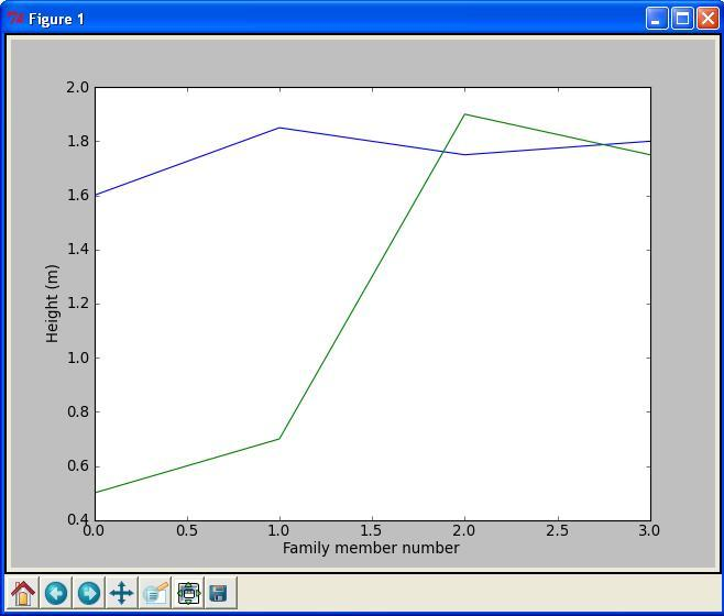
Sometimes you would like to have two or more curves or graphs in the same plot. Assume we have h as above, and also an array H with the heights \( 0.50 \) m, \( 0.70 \) m, \( 1.90 \) m, and \( 1.75 \) m from a family next door. This may be done with the program plot_heights.py given as

from numpy import zeros
import matplotlib.pyplot as plt

h = zeros(4)
h[0] = 1.60; h[1] = 1.85; h[2] = 1.75; h[3] = 1.80
H = zeros(4)
H[0] = 0.50; H[1] = 0.70; H[2] = 1.90; H[3] = 1.75

family_member_no = zeros(4)
family_member_no[0] = 0; family_member_no[1] = 1
family_member_no[2] = 2; family_member_no[3] = 3

plt.plot(family_member_no, h, family_member_no, H)
plt.xlabel('Family member number')
plt.ylabel('Height (m)')
plt.show()

Running the program gives the plot shown in Figure 2.

Alternatively, the two curves could have been plotted in the same plot by use of two plot commands, which gives more freedom as to how the curves appear. To do this, you could plot the first curve by

plot(family_member_no, h)
hold('on')

Then you could (in principle) do a lot of other things in your code, before you plot the second curve by

plot(family_member_no, H)
hold('off')

Notice the use of hold here. hold('on') tells Python to plot also the following curve(s) in the same window. Python does so until it reads hold('off'). If you do not use the hold('on') or hold('off') command, the second plot command will overwrite the first one, i.e., you get only the second curve.

In case you would like the two curves plotted in two separate plots, you can do this by plotting the first curve straightforwardly with

plot(family_member_no, h)

then do other things in your code, before you do

figure()
plot(family_member_no, H)

Note how the graphs are made continuous by Python, drawing straight lines between the four data points of each family. This is the standard way of doing it and was also done when plotting our 1001 height computations with ball_plot.py in the chapter A Python program with vectorization and plotting. However, since there were so many data points then, the curve looked nice and smooth. If preferred, one may also plot only the data points. For example, writing

plot(h, '*')

will mark only the data points with the star symbol. Other symbols like circles etc. may be used as well.

There are many possibilities in Python for adding information to a plot or for changing its appearance. For example, you may add a legend by the instruction

legend('This is some legend')

or you may add a title by

title('This is some title')

The command

axis([xmin, xmax, ymin, ymax])

will define the plotting range for the \( x \) axis to stretch from xmin to xmax and, similarly, the plotting range for the \( y \) axis from ymin to ymax. Saving the figure to file is achieved by the command

savefig('some_plot.png')   # PNG format
savefig('some_plot.pdf')   # PDF format
savefig('some_plot.gif')   # GIF format
savefig('some_plot.eps')   # Encanspulated PostScript format

For the reader who is into linear algebra, it may be useful to know that standard matrix/vector operations are straightforward with arrays, e.g., matrix-vector multiplication. What is needed though, is to create the right variable types (after having imported an appropriate module). For example, assume you would like to calculate the vector \( \bf{y} \) (note that boldface is used for vectors and matrices) as \( \bf{y} = \bf{Ax} \), where \( \bf{A} \) is a \( 2 \times 2 \) matrix and \( \bf{x} \) is a vector. We may do this as illustrated by the program matrix_vector_product.py reading

from numpy import zeros, mat, transpose

x = zeros(2)
x = mat(x)
x = transpose(x)
x[0] = 3;   x[1] = 2   # Pick some values

A = zeros((2,2))
A = mat(A)
A[0,0] = 1;  A[0,1] = 0
A[1,0] = 0;  A[1,1] = 1

# The following gives y = x since A = I, the identity matrix
y = A*x
print y

Here, x is first created as an array, just as we did above. Then the variable type of x is changed to mat, i.e., matrix, by the line x = mat(x). This is followed by a transpose of x from dimension \( 1 \times 2 \) (the default dimension) to \( 2 \times 1 \) with the statement x = transpose(x), before some test values are plugged in. The matrix A is first created as a two dimensional array with A = zeros((2,2)) before conversion and filling in values take place. Finally, the multiplication is performed as y = A*x. Note the number of parentheses when creating the two dimensional array A. Running the program gives the following output on the screen:

[[3.]
 [2.]]

Error messages and warnings

All programmers experience error messages, and usually to a large extent during the early learning process. Sometimes error messages are understandable, sometimes they are not. Anyway, it is important to get used to them. One idea is to start with a program that initially is working, and then deliberately introduce errors in it, one by one. (But remember to take a copy of the original working code!) For each error, you try to run the program to see what Python's response is. Then you know what the problem is and understand what the error message is about. This will greatly help you when you get a similar error message or warning later.

Very often, you will experience that there are errors in the program you have written. This is normal, but frustrating in the beginning. You then have to find the problem, try to fix it, and then run the program again. Typically, you fix one error just to experience that another error is waiting around the corner. However, after some time you start to avoid the most common beginner's errors, and things run more smoothly. The process of finding and fixing errors, called debugging, is very important to learn. There are different ways of doing it too.

A special program (debugger) may be used to help you check (and do) different things in the program you need to fix. A simpler procedure, that often brings you a long way, is to print information to the screen from different places in the program. First of all, this is something you should do (several times) during program development anyway, so that things get checked as you go along. However, if the final program still ends up with error messages, you may save a copy of it, and do some testing on the copy. Useful testing may then be to remove, e.g., the latter half of the program (by inserting comment signs #), and insert print commands at clever places to see what is the case. When the first half looks ok, insert parts of what was removed and repeat the process with the new code. Using simple numbers and doing this in parallel with hand calculations on a piece of paper (for comparison) is often a very good idea.

Python also offers means to detect and handle errors by the program itself! The programmer must then foresee (when writing the code) that there is a potential for error at some particular point. If, for example, some user of the program is asked (by the running program) to provide a number, and intends to give the number 5, but instead writes the word five, the program could run into trouble. A try-exception construction may be used by the programmer to check for such errors and act appropriately (see the chapter Newton's method for an example), avoiding a program crash. This procedure of trying an action and then recovering from trouble, if necessary, is referred to as exception handling and is the modern way of dealing with errors in a program.

When a program finally runs without error messages, it might be tempting to think that Ah..., I am finished!. But no! Then comes program testing, you need to verify that the program does the computations as planned. This is almost an art and may take more time than to develop the program, but the program is useless unless you have much evidence showing that the computations are correct. Also, having a set of (automatic) tests saves huge amounts of time when you further develop the program.

Input data

Computer programs need a set of input data and the purpose is to use these data to compute output data, i.e., results. In the previous program we have specified input data in terms of variables. However, one often wants to get the input through some dialog with the user. Here is one example where the program asks a question, and the user provides an answer by typing on the keyboard:

age = input('What is your age? ')
print "Ok, so you're half way to %d, wow!" % (age*2)

So, after having interpreted and run the first line, Python has established the variable age and assigned your input to it. The second line combines the calculation of twice the age with a message printed on the screen. Try these two lines in a little test program to see for yourself how it works.

The input function is useful for numbers, lists (the chapter Basic constructions), and tuples (the chapter Basic constructions). For pure text, the user must either enclose the input in quotes, or the program must use the raw_input function instead:

name = raw_input('What is your name? ')

There are other ways of providing input to a program as well, e.g., via a graphical interface (as many readers will be used to) or at the command line (i.e., as parameters succeeding, on the same line, the command that starts the program). Reading data from a file is yet another way. Logically, what the program produces when run, e.g. a plot or printout to the screen or a file, is referred to as program output.

Symbolic computations

Even though the main focus in this book is programming of numerical methods, there are occasions where symbolic (also called exact or analytical) operations are useful. Doing symbolic computations means, as the name suggests, that we do computations with the symbols themselves rather than with the numerical values they could represent. Let us illustrate the difference between symbolic and numerical computations with a little example. A numerical computation could be

x = 2
y = 3
z = x*y
print z

which will make the number 6 appear on the screen. A symbolic counterpart of this code could be

from sympy import *
x, y = symbols('x y')
z = x*y
print z

which causes the symbolic result x*y to appear on the screen. Note that no numerical value was assigned to any of the variables in the symbolic computation. Only the symbols were used, as when you do symbolic mathematics by hand on a piece of paper.

Symbolic computations in Python make use of the SymPy package. Each symbol is represented by a standard variable, but the name of the symbol must be declared with Symbol(name) for a single symbol, or symbols(name1 name2 ...) for multiple symbols.. The following script example_symbolic.py is a quick demonstration of some of the basic symbolic operations that are supported in Python.

from sympy import *

x = Symbol('x')
y = Symbol('y')

print 2*x + 3*x - y                # Algebraic computation
print diff(x**2, x)                # Differentiates x**2 wrt. x
print integrate(cos(x), x)         # Integrates cos(x) wrt. x
print simplify((x**2 + x**3)/x**2) # Simplifies expression
print limit(sin(x)/x, x, 0)        # Finds limit of sin(x)/x as x->0
print solve(5*x - 15, x)           # Solves 5*x = 15

Other symbolic calculations like Taylor series expansion, linear algebra (with matrix and vector operations), and (some) differential equation solving are also possible.

Symbolic computations are also readily accessible through the (partly) free online tool WolframAlpha, which applies the very advanced Mathematica package as symbolic engine. The disadvantage with WolframAlpha compared to the SymPy package is that the results cannot automatically be imported into your code and used for further analysis. On the other hand, WolframAlpha has the advantage that it displays many additional mathematical results related to the given problem. For example, if we type 2x + 3x - y in WolframAlpha, it not only simplifies the expression to 5x - y, but it also makes plots of the function \( f(x,y)=5x-y \), solves the equation \( 5x - y = 0 \), and calculates the integral \( \int\int(5x+y)dxdy \). The commercial Pro version can also show a step-by-step of the analytical computations in the problem. You are strongly encouraged to try out these commands in WolframAlpha:

• diff(x^2, x) or diff(x**2, x)
• integrate(cos(x), x)
• simplify((x**2 + x**3)/x**2)
• limit(sin(x)/x, x, 0)
• solve(5*x - 15, x)

Another impressive tool for symbolic computations is Sage, which is a very comprehensive package with the aim of "creating a viable free open source alternative to Magma, Maple, Mathematica and Matlab". Sage is implemented in Python. Projects with extensive symbolic computations will certainly benefit from exploring Sage.

Concluding remarks

The present introductory book just provides a tiny bit of all the functionality that Python has to offer. An important source of information is the official Python documentation website (http://docs.python.org/), which provides a Python tutorial, the Python Library Reference, a Language Reference, and more. Several excellent books are also available (http://wiki.python.org/moin/PythonBooks), but not so many with a scientific computing focus. One exception is Langtangen's comprehensive book A Primer on Scientific Programming with Python, Springer, 2016.

• ← Prev
• Next →