A Python program with vectorization and plotting
We return to the problem where a ball is thrown up in the air and we have a formula for the vertical position \( y \) of the ball. Say we are interested in \( y \) at every milli-second for the first second of the flight. This requires repeating the calculation of \( y=v_0t-0.5gt^2 \) one thousand times.
We will also draw a graph of \( y \) versus \( t \) for \( t\in [0,1] \). Drawing such graphs on a computer essentially means drawing straight lines between points on the curve, so we need many points to make the visual impression of a smooth curve. With one thousand points, as we aim to compute here, the curve looks indeed very smooth.
In Python, the calculations and the visualization of the curve may be done with the program ball_plot.py, reading
from numpy import linspace
import matplotlib.pyplot as plt

v0 = 5
g = 9.81
t = linspace(0, 1, 1001)

y = v0*t - 0.5*g*t**2

plt.plot(t, y)
plt.xlabel('t (s)')
plt.ylabel('y (m)')
plt.show()
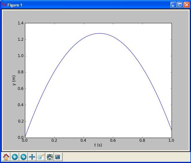
This program produces a plot of the vertical position with time,
as seen in Figure 1.
As you notice, the code lines from the ball.py program
in the chapter A Python program with variables have not changed much, but
the height is now computed and plotted for a thousand points in time!
Let us take a look at the differences between the new program and our previous program. From the top, the first difference we notice are the lines
from numpy import *
from matplotlib.pyplot import *
You see the word import here, so you understand that
numpy must be a library, or module in Python terminology.
This library contains a lot of very useful functionality for
mathematical computing, while the matplotlib.pyplot module
contains functionality for plotting curves.
The above import statement constitutes a quick way
of populating your program with all necessary functionality
for mathematical computing and plotting. However,
we actually make use of only a few functions in the present
program: linspace, plot, xlabel, and ylabel.
Many computer scientists will therefore argue that we should
explicitly import what we need and not everything (the star *):
from numpy import linspace
from matplotlib.pyplot import plot, xlabel, ylabel
Others will claim that we should do a slightly different import and prefix library functions by the library name:
import numpy as np
import matplotlib.pyplot as plt
...
t = np.linspace(0, 1, 1001)
...
plt.plot(t, y)
plt.xlabel('t (s)')
plt.ylabel('y (m)')
We will use all three techniques, and since all of them are in so widespread use, you should be familiar with them too. However, for the most part in this book we shall do
from numpy import *
from matplotlib.pyplot import *
for convenience and for making Python programs that look very similar to their Matlab counterparts.
The function linspace takes \( 3 \) parameters, and is generally called as
linspace(start, stop, n)
This is our first example of a Python function that takes multiple
arguments. The linspace function generates n equally spaced
coordinates, starting with start and ending with stop. The
expression linspace(0, 1, 1001) creates 1001 coordinates between 0
and 1 (including both 0 and 1). The mathematically inclined reader
will notice that 1001 coordinates correspond to 1000 equal-sized
intervals in \( [0,1] \) and that the coordinates are then given by \( t_i =
i/1000 \) (\( i = 0, 1, ..., 1000 \)).
Figure 1: Plot generated by the script ball_plot.py showing the vertical position of the ball at a thousand points in time.
The value returned from linspace (being stored in t) is an array,
i.e., a collection of numbers. When we start computing with this
collection of numbers in the arithmetic expression
v0*t - 0.5*g*t**2, the expression is calculated for
every number in t (i.e., every \( t_i \) for \( i = 0, 1,..., 1000 \)), yielding a similar collection of 1001 numbers in the result y. That is, y is also an array.
This technique of computing all numbers "in one chunk" is referred to
as vectorization. When it can be used, it is very handy, since both
the amount of code and computation time is reduced compared to writing
a corresponding for or while loop (the chapter Basic constructions) for doing the same thing.
The plotting commands are simple:
-
plot(t, y)means plotting all theycoordinates versus all thetcoordinates -
xlabel('t (s)')places the textt (s)on the \( x \) axis -
ylabel('y (m)')places the texty (m)on the \( y \) axis