The composite midpoint method
The idea
Rather than approximating the area under a curve by trapezoids, we can use plain rectangles. It may sound less accurate to use horizontal lines and not skew lines following the function to be integrated, but an integration method based on rectangles (the midpoint method) is in fact slightly more accurate than the one based on trapezoids!
In the midpoint method, we construct a rectangle for every sub-interval where the height equals \( f \) at the midpoint of the sub-interval. Let us do this for four rectangles, using the same sub-intervals as we had for hand calculations with the trapezoidal method: \( [0,0.2) \), \( [0.2,0.6) \), \( [0.6,0.8) \), and \( [0.8,1.0] \). We get $$ \begin{align} \int_0^1 f(t)dt &\approx h_1 f\left(\frac{0 + 0.2}{2}\right) + h_2 f\left(\frac{0.2 + 0.6}{2}\right) \nonumber \\ &+ h_3 f\left(\frac{0.6 + 0.8}{2}\right) + h_4 f\left(\frac{0.8 + 1.0}{2}\right), \tag{3.18} \end{align} $$ where \( h_1 \), \( h_2 \), \( h_3 \), and \( h_4 \) are the widths of the sub-intervals, used previously with the trapezoidal method and defined in (3.10)-(3.13).
Figure 9: Computing approximately the integral of a function as the sum of the areas of the rectangles.
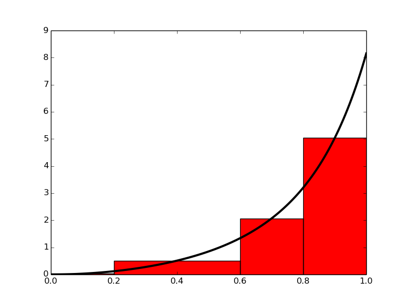
With \( f(t) = 3t^{2}e^{t^3} \), the approximation becomes \( 1.632 \). Compared with the true answer (\( 1.718 \)), this is about \( 5\% \) too small, but it is better than what we got with the trapezoidal method (\( 10\% \)) with the same sub-intervals. More rectangles give a better approximation.
The general formula
Let us derive a formula for the midpoint method based on \( n \) rectangles of equal width: $$ \begin{align} \int_a^b f(x)\,dx &= \int_{x_0}^{x_1} f(x)dx + \int_{x_1}^{x_2} f(x)dx + \ldots + \int_{x_{n-1}}^{x_n} f(x)dx, \nonumber \\ &\approx h f\left(\frac{x_0 + x_1}{2}\right) + h f\left(\frac{x_1 + x_2}{2}\right) + \ldots + h f\left(\frac{x_{n-1} + x_n}{2}\right) , \tag{3.19} \\ &\approx h \left(f\left(\frac{x_0 + x_1}{2}\right) + f\left(\frac{x_1 + x_2}{2}\right) + \ldots + f\left(\frac{x_{n-1} + x_n}{2}\right)\right)\thinspace . \tag{3.20} \end{align} $$ This sum may be written more compactly as $$ \begin{equation} \int_a^b f(x) dx \approx h \sum_{i=0}^{n-1}f(x_i) , \tag{3.21} \end{equation} $$ where \( x_i = \left(a + \frac{h}{2}\right) + ih \).
Implementation
We follow the advice and lessons learned from the implementation of
the trapezoidal method and make a function midpoint(f, a, b, n)
(in a file midpoint.py)
for implementing the general formula (3.21):
def midpoint(f, a, b, n):
    h = float(b-a)/n
    result = 0
    for i in range(n):
        result += f((a + h/2.0) + i*h)
    result *= h
    return result
We can test the function as we explained for the similar trapezoidal
method. The error in our particular problem \( \int_0^1 3t^2e^{t^3}dt \)
with four intervals is now about 0.1 in contrast to 0.2 for the
trapezoidal rule. This is in fact not accidental: one can show
mathematically that the error of the midpoint method is a bit smaller
than for the trapezoidal method. The differences are seldom of any
practical importance, and on a laptop we can easily use \( n=10^6 \) and
get the answer with an error about \( 10^{-12} \) in a couple of seconds.
Comparing the trapezoidal and the midpoint methods
The next example shows how easy we can combine the trapezoidal and midpoint
functions to make a comparison of the two methods in the
file
compare_integration_methods.py:
from trapezoidal import trapezoidal
from midpoint import midpoint
from math import exp

g = lambda y: exp(-y**2)
a = 0
b = 2
print '    n        midpoint          trapezoidal'
for i in range(1, 21):
    n = 2**i
    m = midpoint(g, a, b, n)
    t = trapezoidal(g, a, b, n)
    print '%7d %.16f %.16f' % (n, m, t)
Note the efforts put into nice formatting - the output becomes
    n        midpoint          trapezoidal
      2 0.8842000076332692 0.8770372606158094
      4 0.8827889485397279 0.8806186341245393
      8 0.8822686991994210 0.8817037913321336
     16 0.8821288703366458 0.8819862452657772
     32 0.8820933014203766 0.8820575578012112
     64 0.8820843709743319 0.8820754296107942
    128 0.8820821359746071 0.8820799002925637
    256 0.8820815770754198 0.8820810181335849
    512 0.8820814373412922 0.8820812976045025
   1024 0.8820814024071774 0.8820813674728968
   2048 0.8820813936736116 0.8820813849400392
   4096 0.8820813914902204 0.8820813893068272
   8192 0.8820813909443684 0.8820813903985197
  16384 0.8820813908079066 0.8820813906714446
  32768 0.8820813907737911 0.8820813907396778
  65536 0.8820813907652575 0.8820813907567422
 131072 0.8820813907631487 0.8820813907610036
 262144 0.8820813907625702 0.8820813907620528
 524288 0.8820813907624605 0.8820813907623183
1048576 0.8820813907624268 0.8820813907623890
A visual inspection of the numbers shows how fast the digits stabilize in both methods. It appears that 13 digits have stabilized in the last two rows.
Testing
Problems with brief testing procedures
Testing of the programs for numerical integration has so far employed two strategies. If we have an exact answer, we compute the error and see that increasing \( n \) decreases the error. When the exact answer is not available, we can (as in the comparison example in the previous section) look at the integral values and see that they stabilize as \( n \) grows. Unfortunately, these are very weak test procedures and not at all satisfactory for claiming that the software we have produced is correctly implemented.
To see this, we can introduce a bug in the
application function that calls trapezoidal: instead of
integrating \( 3t^2e^{t^3} \), we write "accidentally" \( 3t^3e^{t^3} \),
but keep the same anti-derivative \( V(t)e^{t^3} \) for computing the
error. With the bug and \( n=4 \), the error is 0.1, but without the bug
the error is 0.2! It is of course completely impossible to tell if
0.1 is the right value of the error. Fortunately, increasing \( n \) shows
that the error stays about 0.3 in the program with the bug, so
the test procedure with increasing \( n \) and checking that the error
decreases points to a problem in the code.
Let us look at another bug, this time in the mathematical algorithm:
instead of computing \( \frac{1}{2}(f(a) + f(b)) \) as we should, we
forget the second \( \frac{1}{2} \) and write 0.5*f(a) + f(b). The error for
\( n=4,40,400 \) when computing
\( \int_{1.1}^{1.9} 3t^2e^{t^3}dt \) goes like \( 1400 \), \( 107 \), \( 10 \),
respectively, which looks promising. The problem is that
the right errors should be \( 369 \), \( 4.08 \), and
\( 0.04 \). That is, the error should be reduced faster in the
correct than in the buggy code. The problem, however, is that it is
reduced in both codes, and we may stop further testing and believe
everything is correctly implemented.
Proper test procedures
There are three serious ways to test the implementation of numerical methods via unit tests:
- Comparing with hand-computed results in a problem with few arithmetic operations, i.e., small \( n \).
- Solving a problem without numerical errors. We know that the trapezoidal rule must be exact for linear functions. The error produced by the program must then be zero (to machine precision).
- Demonstrating correct convergence rates. A strong test when we can compute exact errors, is to see how fast the error goes to zero as \( n \) grows. In the trapezoidal and midpoint rules it is known that the error depends on \( n \) as \( n^{-2} \) as \( n\rightarrow\infty \).
Hand-computed results
Let us use two trapezoids and compute the integral \( \int_0^1v(t) \), \( v(t)=3t^2e^{t^3} \): $$ \frac{1}{2}h(v(0) + v(0.5)) + \frac{1}{2}h(v(0.5)+v(1)) = 2.463642041244344,$$ when \( h=0.5 \) is the width of the two trapezoids. Running the program gives exactly the same results.
Solving a problem without numerical errors
The best unit tests for numerical algorithms involve mathematical problems where we know the numerical result beforehand. Usually, numerical results contain unknown approximation errors, so knowing the numerical result implies that we have a problem where the approximation errors vanish. This feature may be present in very simple mathematical problems. For example, the trapezoidal method is exact for integration of linear functions \( f(x)=ax+b \). We can therefore pick some linear function and construct a test function that checks equality between the exact analytical expression for the integral and the number computed by the implementation of the trapezoidal method.
A specific test case can be \( \int_{1.2}^{4.4} (6x-4)dx \). This integral involves an "arbitrary" interval \( [1.2, 4.4] \) and an "arbitrary" linear function \( f(x) = 6x-4 \). By "arbitrary" we mean expressions where we avoid the special numbers 0 and 1 since these have special properties in arithmetic operations (e.g., forgetting to multiply is equivalent to multiplying by 1, and forgetting to add is equivalent to adding 0).
Demonstrating correct convergence rates
Normally, unit tests must be based on problems where the numerical approximation errors in our implementation remain unknown. However, we often know or may assume a certain asymptotic behavior of the error. We can do some experimental runs with the test problem \( \int_0^1 3t^2e^{t^3}dt \) where \( n \) is doubled in each run: \( n=4,8,16 \). The corresponding errors are then 12%, 3% and 0.77%, respectively. These numbers indicate that the error is roughly reduced by a factor of 4 when doubling \( n \). Thus, the error converges to zero as \( n^{-2} \) and we say that the convergence rate is 2. In fact, this result can also be shown mathematically for the trapezoidal and midpoint method. Numerical integration methods usually have an error that converge to zero as \( n^{-p} \) for some \( p \) that depends on the method. With such a result, it does not matter if we do not know what the actual approximation error is: we know at what rate it is reduced, so running the implementation for two or more different \( n \) values will put us in a position to measure the expected rate and see if it is achieved.
The idea of a corresponding unit test is then to run the algorithm for some \( n \) values, compute the error (the absolute value of the difference between the exact analytical result and the one produced by the numerical method), and check that the error has approximately correct asymptotic behavior, i.e., that the error is proportional to \( n^{-2} \) in case of the trapezoidal and midpoint method.
Let us develop a more precise method for such unit tests based on convergence rates. We assume that the error \( E \) depends on \( n \) according to $$ E = Cn^r,$$
where \( C \) is an unknown constant and \( r \) is the convergence rate. Consider a set of experiments with various \( n \): \( n_0, n_1, n_2, \ldots,n_q \). We compute the corresponding errors \( E_0,\ldots,E_q \). For two consecutive experiments, number \( i \) and \( i-1 \), we have the error model $$ \begin{align} E_{i} &= Cn_{i}^r, \tag{3.22}\\ E_{i-1} &= Cn_{i-1}^r\thinspace . \tag{3.23} \end{align} $$ These are two equations for two unknowns \( C \) and \( r \). We can easily eliminate \( C \) by dividing the equations by each other. Then solving for \( r \) gives $$ \begin{equation} r_{i-1} = \frac{\ln (E_i/E_{i-1})}{\ln (n_i/n_{i-1})}\thinspace . \tag{3.24} \end{equation} $$ We have introduced a subscript \( i-1 \) in \( r \) since the estimated value for \( r \) varies with \( i \). Hopefully, \( r_{i-1} \) approaches the correct convergence rate as the number of intervals increases and \( i\rightarrow q \).
Finite precision of floating-point numbers
The test procedures above lead to comparison of numbers for checking that
calculations were correct.
Such comparison is more complicated than what a newcomer might think.
Suppose we have a calculation a + b and want to check that the
result is what we expect. We start with 1 + 2:
>>> a = 1; b = 2; expected = 3
>>> a + b == expected
True
Then we proceed with 0.1 + 0.2:
>>> a = 0.1; b = 0.2; expected = 0.3
>>> a + b == expected
False
So why is \( 0.1 + 0.2 \neq 0.3 \)? The reason is that real numbers cannot in general be exactly represented on a computer. They must instead be approximated by a floating-point number that can only store a finite amount of information, usually about 17 digits of a real number. Let us print 0.1, 0.2, 0.1 + 0.2, and 0.3 with 17 decimals:
>>> print '%.17f\n%.17f\n%.17f\n%.17f' % (0.1, 0.2, 0.1 + 0.2, 0.3)
0.10000000000000001
0.20000000000000001
0.30000000000000004
0.29999999999999999
We see that all of the numbers have an inaccurate digit in the 17th decimal place. Because 0.1 + 0.2 evaluates to 0.30000000000000004 and 0.3 is represented as 0.29999999999999999, these two numbers are not equal. In general, real numbers in Python have (at most) 16 correct decimals.
When we compute with real numbers, these numbers are inaccurately represented on the computer, and arithmetic operations with inaccurate numbers lead to small rounding errors in the final results. Depending on the type of numerical algorithm, the rounding errors may or may not accumulate.
If we cannot make tests like 0.1 + 0.2 == 0.3, what should we then do?
The answer is that we must accept some small inaccuracy and make
a test with a tolerance. Here is the recipe:
>>> a = 0.1; b = 0.2; expected = 0.3
>>> computed = a + b
>>> diff = abs(expected - computed)
>>> tol = 1E-15
>>> diff < tol
True
Here we have set the tolerance for comparison to \( 10^{-15} \), but
calculating 0.3 - (0.1 + 0.2) shows that it equals
-5.55e-17, so a lower tolerance
could be used in this particular example. However, in other calculations
we have little idea about how accurate the answer is (there could be
accumulation of rounding errors in more complicated algorithms),
so \( 10^{-15} \) or \( 10^{-14} \) are robust values.
As we demonstrate below, these tolerances depend on the magnitude of
the numbers in the calculations.
Doing an experiment with \( 10^k + 0.3 - (10^k + 0.1 + 0.2) \) for \( k=1,\ldots,10 \) shows that the answer (which should be zero) is around \( 10^{16-k} \). This means that the tolerance must be larger if we compute with larger numbers. Setting a proper tolerance therefore requires some experiments to see what level of accuracy one can expect. A way out of this difficulty is to work with relative instead of absolute differences. In a relative difference we divide by one of the operands, e.g., $$ a = 10^k + 0.3,\quad b = (10^k + 0.1 + 0.2),\quad c = \frac{a - b}{a}\thinspace .$$ Computing this \( c \) for various \( k \) shows a value around \( 10^{-16} \). A safer procedure is thus to use relative differences.
Constructing unit tests and writing test functions
Python has several frameworks for automatically running and checking a potentially very large number of tests for parts of your software by one command. This is an extremely useful feature during program development: whenever you have done some changes to one or more files, launch the test command and make sure nothing is broken because of your edits.
The test frameworks nose and py.test are particularly attractive
as they are very easy to use.
Tests are placed in special test functions
that the frameworks can recognize and run for you. The requirements
to a test function are simple:
- the name must start with
test_ - the test function cannot have any arguments
- the tests inside test functions must be boolean expressions
- a boolean expression
bmust be tested withassert b, msg, wheremsgis an optional object (string or number) to be written out whenbis false
def add(a, b):
    return a + b
A corresponding test function can then be
def test_add()
    expected = 1 + 1
    computed = add(1, 1)
    assert computed == expected, '1+1=%g' % computed
Test functions can be in any program file or in separate files,
typically with names starting with test. You can also collect
tests in subdirectories: running py.test -s -v will actually
run all tests in all test*.py files in all subdirectories, while
nosetests -s -v restricts the attention to subdirectories whose
names start with test or end with _test or _tests.
As long as we add integers, the equality test in the test_add
function is appropriate, but if we try to call add(0.1, 0.2)
instead, we will face the rounding error problems explained in
the section Finite precision of floating-point numbers, and we must use a test
with tolerance instead:
def test_add()
    expected = 0.3
    computed = add(0.1, 0.2)
    tol = 1E-14
    diff = abs(expected - computed)
    assert diff < tol, 'diff=%g' % diff
Below we shall write test functions for each of the three test
procedures we suggested: comparison with hand calculations,
checking problems that can be exactly solved, and checking convergence
rates. We stick to testing the trapezoidal integration code and collect all
test functions in one common file by the name test_trapezoidal.py.
Hand-computed numerical results
Our previous hand calculations for two trapezoids can be checked against
the trapezoidal function inside a test function
(in a file test_trapezoidal.py):
from trapezoidal import trapezoidal

def test_trapezoidal_one_exact_result():
    """Compare one hand-computed result."""
    from math import exp
    v = lambda t: 3*(t**2)*exp(t**3)
    n = 2
    computed = trapezoidal(v, 0, 1, n)
    expected = 2.463642041244344
    error = abs(expected - computed)
    tol = 1E-14
    success = error < tol
    msg = 'error=%g > tol=%g' % (errror, tol)
    assert success, msg
Note the importance of checking err against exact with a tolerance:
rounding errors from the arithmetics inside trapezoidal will not
make the result exactly like the hand-computed one. The size of
the tolerance is here set to \( 10^{-14} \), which is a kind of all-round
value for computations with numbers not deviating much from unity.
Solving a problem without numerical errors
We know that the trapezoidal rule is exact for linear integrands. Choosing the integral \( \int_{1.2}^{4.4} (6x-4)dx \) as test case, the corresponding test function for this unit test may look like
def test_trapezoidal_linear():
    """Check that linear functions are integrated exactly."""
    f = lambda x: 6*x - 4
    F = lambda x: 3*x**2 - 4*x  # Anti-derivative
    a = 1.2; b = 4.4
    expected = F(b) - F(a)
    tol = 1E-14
    for n in 2, 20, 21:
        computed = trapezoidal(f, a, b, n)
        error = abs(expected - computed)
        success = error < tol
        msg = 'n=%d, err=%g' % (n, error)
        assert success, msg
Demonstrating correct convergence rates
In the present example with integration, it is known that the approximation errors in the trapezoidal rule are proportional to \( n^{-2} \), \( n \) being the number of subintervals used in the composite rule.
Computing convergence rates requires somewhat more tedious programming than the previous tests, but can be applied to more general integrands. The algorithm typically goes like
- for \( i=0,1,2,\ldots,q \)
- \( n_i = 2^{i+1} \)
- Compute integral with \( n_i \) intervals
- Compute the error \( E_i \)
- Estimate \( r_i \) from (3.24) if \( i>0 \)
def convergence_rates(f, F, a, b, num_experiments=14):
    from math import log
    from numpy import zeros
    expected = F(b) - F(a)
    n = zeros(num_experiments, dtype=int)
    E = zeros(num_experiments)
    r = zeros(num_experiments-1)
    for i in range(num_experiments):
        n[i] = 2**(i+1)
        computed = trapezoidal(f, a, b, n[i])
        E[i] = abs(expected - computed)
        if i > 0:
            r_im1 = log(E[i]/E[i-1])/log(float(n[i])/n[i-1])
            r[i-1] = float('%.2f' % r_im1) # Truncate to two decimals
    return r
Making a test function is a matter of choosing f, F, a, and b,
and then checking the value of \( r_i \) for the largest \( i \):
def test_trapezoidal_conv_rate():
    """Check empirical convergence rates against the expected -2."""
    from math import exp
    v = lambda t: 3*(t**2)*exp(t**3)
    V = lambda t: exp(t**3)
    a = 1.1; b = 1.9
    r = convergence_rates(v, V, a, b, 14)
    print r
    tol = 0.01
    msg = str(r[-4:])  # show last 4 estimated rates
    assert (abs(r[-1]) - 2) < tol, msg
Running the test shows that all \( r_i \), except the first one, equal the target limit 2 within two decimals. This observation suggest a tolerance of \( 10^{-2} \).
The typical workflow with Git goes as follows.
- Before you start working with files, make sure you have the latest
version of them by running
git pull. - Edit files, remove or create files (new files must be registered
by
git add). - When a natural piece of work is done, commit your changes by the
git commitcommand. - Implement your changes also in the cloud by doing
git push.
Vectorization
The functions midpoint and trapezoid usually run fast in Python
and compute an integral to a satisfactory precision within a
fraction of a second. However, long loops in Python may run slowly in more
complicated implementations. To increase the speed, the loops
can be replaced by vectorized code. The integration functions constitute
a simple and good example to illustrate how to vectorize loops.
We have already seen simple examples on vectorization in the section A Python program with vectorization and plotting when we could evaluate a mathematical function \( f(x) \) for a large number of \( x \) values stored in an array. Basically, we can write
def f(x):
    return exp(-x)*sin(x) + 5*x

from numpy import exp, sin, linspace
x = linspace(0, 4, 101)  # coordinates from 100 intervals on [0, 4]
y = f(x)                 # all points evaluated at once
The result y is the array that would be computed if we ran a
for loop over the individual
x values and called f for each value. Vectorization essentially
eliminates this loop in Python (i.e., the looping over x and application
of f to each x value are instead performed
in a library with fast, compiled code).
Vectorizing the midpoint rule
The aim of vectorizing the midpoint and trapezoidal functions is
also to remove the explicit loop in Python.
We start with vectorizing the midpoint function since trapezoid
is not equally straightforward. The fundamental ideas of the vectorized
algorithm are to
- compute all the evaluation points in one array
x - call
f(x)to produce an array of corresponding function values - use the
sumfunction to sum thef(x)values
x = linspace(a+h/2, b-h/2, n).
Given that the
Python implementation f of the mathematical function \( f \) works with
an array argument,
which is very often the case in Python,
f(x) will produce all the function values in an
array. The array elements are then summed up by sum: sum(f(x)). This
sum is to be multiplied by the rectangle width \( h \) to produce
the integral value. The complete function is listed below.
from numpy import linspace, sum

def midpoint(f, a, b, n):
    h = float(b-a)/n
    x = linspace(a + h/2, b - h/2, n)
    return h*sum(f(x))
The code is found in the file integration_methods_vec.py.
Let us test the code interactively in a Python shell to compute
\( \int_0^1 3t^2dt \). The file with the code above has the name
integration_methods_vec.py and is a valid module from which we
can import the vectorized function:
>>> from integration_methods_vec import midpoint
>>> from numpy import exp
>>> v = lambda t: 3*t**2*exp(t**3)
>>> midpoint(v, 0, 1, 10)
1.7014827690091872
Note the necessity to use exp from numpy: our v function will
be called with x as an array, and the exp function must be
capable of working with an array.
The vectorized code performs all loops very efficiently in compiled code, resulting in much faster execution. Moreover, many readers of the code will also say that the algorithm looks clearer than in the loop-based implementation.
Vectorizing the trapezoidal rule
We can use the same approach to vectorize the trapezoid function.
However, the trapezoidal rule performs a sum where the end points
have different weight. If we do sum(f(x)), we get the end points
f(a) and f(b) with weight unity instead of one half. A remedy
is to subtract the error from sum(f(x)): sum(f(x)) - 0.5*f(a) - 0.5*f(b).
The vectorized version of the trapezoidal method then becomes
def trapezoidal(f, a, b, n):
    h = float(b-a)/n
    x = linspace(a, b, n+1)
    s = sum(f(x)) - 0.5*f(a) - 0.5*f(b)
    return h*s
Measuring computational speed
Now that we have created faster, vectorized versions of functions in
the previous section, it is interesting to measure how much faster
they are. The purpose of the present section is therefore to
explain how we can record the CPU time consumed by a function so
we can answer this question.
There are many techniques for measuring the CPU time in Python,
and here we shall
just explain the simplest and most convenient one: the %timeit
command in IPython. The following interactive session should
illustrate a competition where the vectorized versions of the
functions are supposed to win:
In [1]: from integration_methods_vec import midpoint as midpoint_vec

In [3]: from midpoint import midpoint

In [4]: from numpy import exp

In [5]: v = lambda t: 3*t**2*exp(t**3)

In [6]: %timeit midpoint_vec(v, 0, 1, 1000000)
1 loops, best of 3: 379 ms per loop

In [7]: %timeit midpoint(v, 0, 1, 1000000)
1 loops, best of 3: 8.17 s per loop

In [8]: 8.17/(379*0.001)    # efficiency factor
Out[8]: 21.556728232189972
We see that the vectorized version is about 20 times faster: 379 ms versus 8.17 s. The results for the trapezoidal method are very similar, and the factor of about 20 is independent of the number of intervals.
Double and triple integrals
The midpoint rule for a double integral
Given a double integral over a rectangular domain \( [a,b]\times [c,d] \), $$ \int_a^b \int_c^d f(x,y) dydx,$$ how can we approximate this integral by numerical methods?
Derivation via one-dimensional integrals
Since we know how to deal with integrals in one variable, a fruitful approach is to view the double integral as two integrals, each in one variable, which can be approximated numerically by previous one-dimensional formulas. To this end, we introduce a help function \( g(x) \) and write $$ \int_a^b \int_c^d f(x,y) dydx = \int_a^b g(x)dx,\quad g(x) = \int_c^d f(x,y) dy\thinspace .$$ Each of the integrals $$ \int_a^b g(x)dx,\quad g(x) = \int_c^d f(x,y) dy$$ can be discretized by any numerical integration rule for an integral in one variable. Let us use the midpoint method (3.21) and start with \( g(x)=\int_c^d f(x,y)dy \). We introduce \( n_y \) intervals on \( [c,d] \) with length \( h_y \). The midpoint rule for this integral then becomes $$ g(x) = \int_c^d f(x,y) dy \approx h_y \sum_{j=0}^{n_y-1} f(x,y_j), \quad y_j = c + \frac{1}{2}{h_y} + jh_y \thinspace . $$ The expression looks somewhat different from (3.21), but that is because of the notation: since we integrate in the \( y \) direction and will have to work with both \( x \) and \( y \) as coordinates, we must use \( n_y \) for \( n \), \( h_y \) for \( h \), and the counter \( i \) is more naturally called \( j \) when integrating in \( y \). Integrals in the \( x \) direction will use \( h_x \) and \( n_x \) for \( h \) and \( n \), and \( i \) as counter.
The double integral is \( \int_a^b g(x)dx \), which can be approximated by the midpoint method: $$ \int_a^b g(x)dx \approx h_x \sum_{i=0}^{n_x-1} g(x_i),\quad x_i=a + \frac{1}{2}{h_x} + ih_x\thinspace .$$ Putting the formulas together, we arrive at the composite midpoint method for a double integral: $$ \begin{align} \int_a^b \int_c^d f(x,y) dydx &\approx h_x \sum_{i=0}^{n_x-1} h_y \sum_{j=0}^{n_y-1} f(x_i,y_j)\nonumber\\ &= h_xh_y \sum_{i=0}^{n_x-1} \sum_{j=0}^{n_y-1} f(a + \frac{h_x}{2} + ih_x, c + \frac{h_y}{2} + jh_y)\thinspace . \tag{3.25} \end{align} $$
Direct derivation
The formula (3.25) can also be derived directly in the two-dimensional case by applying the idea of the midpoint method. We divide the rectangle \( [a,b]\times [c,d] \) into \( n_x\times n_y \) equal-sized cells. The idea of the midpoint method is to approximate \( f \) by a constant over each cell, and evaluate the constant at the midpoint. Cell \( (i,j) \) occupies the area $$ [a+ih_x,a+(i+1)h_x]\times [c+jh_y, c+ (j+1)h_y],$$ and the midpoint is \( (x_i,y_j) \) with $$ x_i=a + ih_x + \frac{1}{2}{h_x} ,\quad y_j = c + jh_y + \frac{1}{2}{h_y} \thinspace .$$ The integral over the cell is therefore \( h_xh_y f(x_i,y_j) \), and the total double integral is the sum over all cells, which is nothing but formula (3.25).
Programming a double sum
The formula (3.25) involves a double sum, which is normally implemented as a double for loop. A Python function implementing (3.25) may look like
def midpoint_double1(f, a, b, c, d, nx, ny):
    hx = (b - a)/float(nx)
    hy = (d - c)/float(ny)
    I = 0
    for i in range(nx):
        for j in range(ny):
            xi = a + hx/2 + i*hx
            yj = c + hy/2 + j*hy
            I += hx*hy*f(xi, yj)
    return I
If this function is stored in a module file midpoint_double.py, we can compute some integral, e.g., \( \int_2^3\int_0^2 (2x + y)dxdy=9 \) in an interactive shell and demonstrate that the function computes the right number:
>>> from midpoint_double import midpoint_double1
>>> def f(x, y):
...     return 2*x + y
...
>>> midpoint_double1(f, 0, 2, 2, 3, 5, 5)
9.0
Reusing code for one-dimensional integrals
It is very natural to write a two-dimensional midpoint method as we did in
function midpoint_double1 when we have the formula (3.25). However, we could alternatively ask, much as we did in the mathematics,
can we reuse a well-tested implementation for one-dimensional integrals
to compute double integrals? That is, can we use function midpoint
def midpoint(f, a, b, n):
    h = float(b-a)/n
    result = 0
    for i in range(n):
        result += f((a + h/2.0) + i*h)
    result *= h
    return result
from the section Implementation "twice"? The answer is yes, if we think as we did in the mathematics: compute the double integral as a midpoint rule for integrating \( g(x) \) and define \( g(x_i) \) in terms of a midpoint rule over \( f \) in the \( y \) coordinate. The corresponding function has very short code:
def midpoint_double2(f, a, b, c, d, nx, ny):
    def g(x):
        return midpoint(lambda y: f(x, y), c, d, ny)

    return midpoint(g, a, b, nx)
The important advantage of this implementation is that we reuse a well-tested function for the standard one-dimensional midpoint rule and that we apply the one-dimensional rule exactly as in the mathematics.
Verification via test functions
How can we test that our functions for the double integral work? The best unit test is to find a problem where the numerical approximation error vanishes because then we know exactly what the numerical answer should be. The midpoint rule is exact for linear functions, regardless of how many subinterval we use. Also, any linear two-dimensional function \( f(x,y)=px+qy+r \) will be integrated exactly by the two-dimensional midpoint rule. We may pick \( f(x,y)=2x+y \) and create a proper test function that can automatically verify our two alternative implementations of the two-dimensional midpoint rule. To compute the integral of \( f(x,y) \) we take advantage of SymPy to eliminate the possibility of errors in hand calculations. The test function becomes
def test_midpoint_double():
    """Test that a linear function is integrated exactly."""
    def f(x, y):
        return 2*x + y

    a = 0;  b = 2;  c = 2;  d = 3
    import sympy
    x, y = sympy.symbols('x  y')
    I_expected = sympy.integrate(f(x, y), (x, a, b), (y, c, d))
    # Test three cases: nx < ny, nx = ny, nx > ny
    for nx, ny in (3, 5), (4, 4), (5, 3):
        I_computed1 = midpoint_double1(f, a, b, c, d, nx, ny)
        I_computed2 = midpoint_double2(f, a, b, c, d, nx, ny)
        tol = 1E-14
        #print I_expected, I_computed1, I_computed2
        assert abs(I_computed1 - I_expected) < tol
        assert abs(I_computed2 - I_expected) < tol
test_midpoint_double function
and nothing happens, our implementations
are correct. However, it is somewhat annoying to have a function that
is completely silent when it works - are we sure all things are properly
computed? During development it is therefore highly recommended to insert
a print statement such that we can monitor the calculations and be
convinced that the test function does what we want. Since a test
function should not have any print statement, we simply comment it out as
we have done in the function listed above.
The trapezoidal method can be used as alternative for the midpoint method. The derivation of a formula for the double integral and the implementations follow exactly the same ideas as we explained with the midpoint method, but there are more terms to write in the formulas. Exercise 42: Derive the trapezoidal rule for a double integral asks you to carry out the details. That exercise is a very good test on your understanding of the mathematical and programming ideas in the present section.
The midpoint rule for a triple integral
Theory
Once a method that works for a one-dimensional problem is generalized to two dimensions, it is usually quite straightforward to extend the method to three dimensions. This will now be demonstrated for integrals. We have the triple integral $$ \int_{a}^{b} \int_c^d \int_e^f g(x,y,z) dzdydx$$ and want to approximate the integral by a midpoint rule. Following the ideas for the double integral, we split this integral into one-dimensional integrals: $$ \begin{align*} p(x,y) &= \int_e^f g(x,y,z) dz\\ q(x) &= \int_c^d p(x,y) dy\\ \int_{a}^{b} \int_c^d \int_e^f g(x,y,z) dzdydx &= \int_a^b q(x)dx \end{align*} $$ For each of these one-dimensional integrals we apply the midpoint rule: $$ \begin{align*} p(x,y) = \int_e^f g(x,y,z) dz &\approx \sum_{k=0}^{n_z-1} g(x,y,z_k), \\ q(x) = \int_c^d p(x,y) dy &\approx \sum_{j=0}^{n_y-1} p(x,y_j), \\ \int_{a}^{b} \int_c^d \int_e^f g(x,y,z) dzdydx = \int_a^b q(x)dx &\approx \sum_{i=0}^{n_x-1} q(x_i), \end{align*} $$ where $$ z_k=e + \frac{1}{2}h_z + kh_z,\quad y_j=c + \frac{1}{2}h_y + jh_y \quad x_i=a + \frac{1}{2}h_x + ih_x \thinspace . $$ Starting with the formula for \( \int_{a}^{b} \int_c^d \int_e^f g(x,y,z) dzdydx \) and inserting the two previous formulas gives $$ \begin{align} & \int_{a}^{b} \int_c^d \int_e^f g(x,y,z)\, dzdydx\approx\nonumber\\ & h_xh_yh_z \sum_{i=0}^{n_x-1}\sum_{j=0}^{n_y-1}\sum_{k=0}^{n_z-1} g(a + \frac{1}{2}h_x + ih_x, c + \frac{1}{2}h_y + jh_y, e + \frac{1}{2}h_z + kh_z)\thinspace . \tag{3.26} \end{align} $$ Note that we may apply the ideas under Direct derivation at the end of the section The midpoint rule for a double integral to arrive at (3.26) directly: divide the domain into \( n_x\times n_y\times n_z \) cells of volumes \( h_xh_yh_z \); approximate \( g \) by a constant, evaluated at the midpoint \( (x_i,y_j,z_k) \), in each cell; and sum the cell integrals \( h_xh_yh_zg(x_i,y_j,z_k) \).
Implementation
We follow the ideas for the implementations of the midpoint rule for a double integral. The corresponding functions are shown below and found in the file midpoint_triple.py.
def midpoint_triple1(g, a, b, c, d, e, f, nx, ny, nz):
    hx = (b - a)/float(nx)
    hy = (d - c)/float(ny)
    hz = (f - e)/float(nz)
    I = 0
    for i in range(nx):
        for j in range(ny):
            for k in range(nz):
                xi = a + hx/2 + i*hx
                yj = c + hy/2 + j*hy
                zk = e + hz/2 + k*hz
                I += hx*hy*hz*g(xi, yj, zk)
    return I

def midpoint(f, a, b, n):
    h = float(b-a)/n
    result = 0
    for i in range(n):
        result += f((a + h/2.0) + i*h)
    result *= h
    return result

def midpoint_triple2(g, a, b, c, d, e, f, nx, ny, nz):
    def p(x, y):
        return midpoint(lambda z: g(x, y, z), e, f, nz)

    def q(x):
        return midpoint(lambda y: p(x, y), c, d, ny)

    return midpoint(q, a, b, nx)

def test_midpoint_triple():
    """Test that a linear function is integrated exactly."""
    def g(x, y, z):
        return 2*x + y - 4*z

    a = 0;  b = 2;  c = 2;  d = 3;  e = -1;  f = 2
    import sympy
    x, y, z = sympy.symbols('x y z')
    I_expected = sympy.integrate(
        g(x, y, z), (x, a, b), (y, c, d), (z, e, f))
    for nx, ny, nz in (3, 5, 2), (4, 4, 4), (5, 3, 6):
        I_computed1 = midpoint_triple1(
            g, a, b, c, d, e, f, nx, ny, nz)
        I_computed2 = midpoint_triple2(
            g, a, b, c, d, e, f, nx, ny, nz)
        tol = 1E-14
        print I_expected, I_computed1, I_computed2
        assert abs(I_computed1 - I_expected) < tol
        assert abs(I_computed2 - I_expected) < tol

if __name__ == '__main__':
    test_midpoint_triple()
Monte Carlo integration for complex-shaped domains
Repeated use of one-dimensional integration rules to handle double and triple integrals constitute a working strategy only if the integration domain is a rectangle or box. For any other shape of domain, completely different methods must be used. A common approach for two- and three-dimensional domains is to divide the domain into many small triangles or tetrahedra and use numerical integration methods for each triangle or tetrahedron. The overall algorithm and implementation is too complicated to be addressed in this book. Instead, we shall employ an alternative, very simple and general method, called Monte Carlo integration. It can be implemented in half a page of code, but requires orders of magnitude more function evaluations in double integrals compared to the midpoint rule.
However, Monte Carlo integration is much more computationally efficient than the midpoint rule when computing higher-dimensional integrals in more than three variables over hypercube domains. Our ideas for double and triple integrals can easily be generalized to handle an integral in \( m \) variables. A midpoint formula then involves \( m \) sums. With \( n \) cells in each coordinate direction, the formula requires \( n^m \) function evaluations. That is, the computational work explodes as an exponential function of the number of space dimensions. Monte Carlo integration, on the other hand, does not suffer from this explosion of computational work and is the preferred method for computing higher-dimensional integrals. So, it makes sense in a chapter on numerical integration to address Monte Carlo methods, both for handling complex domains and for handling integrals with many variables.
The Monte Carlo integration algorithm
The idea of Monte Carlo integration of \( \int_a^b f(x)dx \) is to use the mean-value theorem from calculus, which states that the integral \( \int_a^b f(x)dx \) equals the length of the integration domain, here \( b-a \), times the average value of \( f \), \( \bar f \), in \( [a,b] \). The average value can be computed by sampling \( f \) at a set of random points inside the domain and take the mean of the function values. In higher dimensions, an integral is estimated as the area/volume of the domain times the average value, and again one can evaluate the integrand at a set of random points in the domain and compute the mean value of those evaluations.
Let us introduce some quantities to help us make the specification of the integration algorithm more precise. Suppose we have some two-dimensional integral $$ \int_\Omega f(x,y)dxdx, $$ where \( \Omega \) is a two-dimensional domain defined via a help function \( g(x,y) \): $$ \Omega = \{ (x,y)\,|\, g(x,y) \geq 0\} $$ That is, points \( (x,y) \) for which \( g(x,y)\geq 0 \) lie inside \( \Omega \), and points for which \( g(x,y) < \Omega \) are outside \( \Omega \). The boundary of the domain \( \partial\Omega \) is given by the implicit curve \( g(x,y)=0 \). Such formulations of geometries have been very common during the last couple of decades, and one refers to \( g \) as a level-set function and the boundary \( g=0 \) as the zero-level contour of the level-set function. For simple geometries one can easily construct \( g \) by hand, while in more complicated industrial applications one must resort to mathematical models for constructing \( g \).
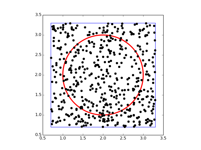
Let \( A(\Omega) \) be the area of a domain \( \Omega \). We can estimate the integral by this Monte Carlo integration method:
- embed the geometry \( \Omega \) in a rectangular area \( R \)
- draw a large number of random points \( (x,y) \) in \( R \)
- count the fraction \( q \) of points that are inside \( \Omega \)
- approximate \( A(\Omega)/A(R) \) by \( q \), i.e., set \( A(\Omega) = qA(R) \)
- evaluate the mean of \( f \), \( \bar f \), at the points inside \( \Omega \)
- estimate the integral as \( A(\Omega)\bar f \)
To get an idea of the method, consider a circular domain \( \Omega \) embedded in a rectangle as shown below. A collection of random points is illustrated by black dots.
Implementation
A Python function implementing \( \int_\Omega f(x,y)dxdy \) can be written like this:
import numpy as np

def MonteCarlo_double(f, g, x0, x1, y0, y1, n):
    """
    Monte Carlo integration of f over a domain g>=0, embedded
    in a rectangle [x0,x1]x[y0,y1]. n^2 is the number of
    random points.
    """
    # Draw n**2 random points in the rectangle
    x = np.random.uniform(x0, x1, n)
    y = np.random.uniform(y0, y1, n)
    # Compute sum of f values inside the integration domain
    f_mean = 0
    num_inside = 0   # number of x,y points inside domain (g>=0)
    for i in range(len(x)):
        for j in range(len(y)):
            if g(x[i], y[j]) >= 0:
                num_inside += 1
                f_mean += f(x[i], y[j])
    f_mean = f_mean/float(num_inside)
    area = num_inside/float(n**2)*(x1 - x0)*(y1 - y0)
    return area*f_mean
(See the file MC_double.py.)
Verification
A simple test case is to check the area of a rectangle \( [0,2]\times[3,4.5] \) embedded in a rectangle \( [0,3]\times [2,5] \). The right answer is 3, but Monte Carlo integration is, unfortunately, never exact so it is impossible to predict the output of the algorithm. All we know is that the estimated integral should approach 3 as the number of random points goes to infinity. Also, for a fixed number of points, we can run the algorithm several times and get different numbers that fluctuate around the exact value, since different sample points are used in different calls to the Monte Carlo integration algorithm.
The area of the rectangle can be computed by the integral \( \int_0^2\int_3^{4.5}
dydx \), so in this case we identify
\( f(x,y)=1 \), and the \( g \) function can be specified as (e.g.)
1 if \( (x,y) \) is inside \( [0,2]\times[3,4.5] \) and \( -1 \) otherwise.
Here is an example on how we can utilize the MonteCarlo_double
function to compute the area for different number of samples:
>>> from MC_double import MonteCarlo_double
>>> def g(x, y):
...     return (1 if (0 <= x <= 2 and 3 <= y <= 4.5) else -1)
...
>>> MonteCarlo_double(lambda x, y: 1, g, 0, 3, 2, 5, 100)
2.9484
>>> MonteCarlo_double(lambda x, y: 1, g, 0, 3, 2, 5, 1000)
2.947032
>>> MonteCarlo_double(lambda x, y: 1, g, 0, 3, 2, 5, 1000)
3.0234600000000005
>>> MonteCarlo_double(lambda x, y: 1, g, 0, 3, 2, 5, 2000)
2.9984580000000003
>>> MonteCarlo_double(lambda x, y: 1, g, 0, 3, 2, 5, 2000)
3.1903469999999996
>>> MonteCarlo_double(lambda x, y: 1, g, 0, 3, 2, 5, 5000)
2.986515
We see that the values fluctuate around 3, a fact that supports a correct implementation, but in principle, bugs could be hidden behind the inaccurate answers.
It is mathematically known that the standard deviation of the Monte Carlo estimate of an integral converges as \( n^{-1/2} \), where \( n \) is the number of samples. This kind of convergence rate estimate could be used to verify the implementation, but this topic is beyond the scope of this book.
Test function for function with random numbers
To make a test function, we need a unit test that has identical
behavior each time we run the test. This seems difficult when random
numbers are involved, because these numbers are different every time
we run the algorithm, and each run hence produces a (slightly)
different result. A standard way to test algorithms involving random
numbers is to fix the seed of the random number generator. Then the
sequence of numbers is the same every time we run the algorithm.
Assuming that the MonteCarlo_double function works, we fix the seed,
observe a certain result, and take this result as the correct
result. Provided the test function always uses this seed, we should
get exactly this result every time the MonteCarlo_double function is
called. Our test function can then be written as shown below.
def test_MonteCarlo_double_rectangle_area():
    """Check the area of a rectangle."""
    def g(x, y):
        return (1 if (0 <= x <= 2 and 3 <= y <= 4.5) else -1)

    x0 = 0;  x1 = 3;  y0 = 2;  y1 = 5  # embedded rectangle
    n = 1000
    np.random.seed(8)      # must fix the seed!
    I_expected = 3.121092  # computed with this seed
    I_computed = MonteCarlo_double(
        lambda x, y: 1, g, x0, x1, y0, y1, n)
    assert abs(I_expected - I_computed) < 1E-14
(See the file MC_double.py.)
Integral over a circle
The test above involves a trivial function \( f(x,y)=1 \). We should also test a non-constant \( f \) function and a more complicated domain. Let \( \Omega \) be a circle at the origin with radius 2, and let \( f=\sqrt{x^2 + y^2} \). This choice makes it possible to compute an exact result: in polar coordinates, \( \int_\Omega f(x,y)dxdy \) simplifies to \( 2\pi\int_0^2 r^2dr = 16\pi/3 \). We must be prepared for quite crude approximations that fluctuate around this exact result. As in the test case above, we experience better results with larger number of points. When we have such evidence for a working implementation, we can turn the test into a proper test function. Here is an example:
def test_MonteCarlo_double_circle_r():
    """Check the integral of r over a circle with radius 2."""
    def g(x, y):
        xc, yc = 0, 0  # center
        R = 2          # radius
        return  R**2 - ((x-xc)**2 + (y-yc)**2)

    # Exact: integral of r*r*dr over circle with radius R becomes
    # 2*pi*1/3*R**3
    import sympy
    r = sympy.symbols('r')
    I_exact = sympy.integrate(2*sympy.pi*r*r, (r, 0, 2))
    print 'Exact integral:', I_exact.evalf()
    x0 = -2;  x1 = 2;  y0 = -2;  y1 = 2
    n = 1000
    np.random.seed(6)
    I_expected = 16.7970837117376384  # Computed with this seed
    I_computed = MonteCarlo_double(
        lambda x, y: np.sqrt(x**2 + y**2),
        g, x0, x1, y0, y1, n)
    print 'MC approximation %d samples): %.16f' % (n**2, I_computed)
    assert abs(I_expected - I_computed) < 1E-15
(See the file MC_double.py.)