This chapter is taken from the book A Primer on Scientific Programming with Python by H. P. Langtangen, 5th edition, Springer, 2016.
Summary
Chapter topics
Drawing random numbers
Random numbers can be scattered throughout an interval in various ways, specified by the distribution of the numbers. We have considered a uniform distribution (the section Uniformly distributed random numbers) and a normal (or Gaussian) distribution (the section The Gaussian or normal distribution).
The table below shows the syntax for generating
random numbers of these two distributions, using either the standard
scalar random module in Python or the vectorized numpy.random
module. Here,
N is the array length in vectorized drawing,
while m and s represent the mean and standard deviation
values of a normal distribution. Functions from the standard random
module appear in the middle column, while the corresponding
functions from numpy.random
are listed in the right column.
| Functionality | Python's random | numpy.random |
| uniform numbers in \( [0,1) \) | random() | random(N) |
| uniform numbers in \( [a,b) \) | uniform(a, b) | uniform(a, b, N) |
| integers in \( [a,b] \) | randint(a, b) | randint(a, b+1, N) |
| integers in \( [a,b] \) | random_integers(a, b, N) | |
| Gaussian numbers | gauss(m, s) | normal(m, s, N) |
set seed (i) | seed(i) | seed(i) |
| shuffle list in-place | shuffle(a) | shuffle(a) |
| choose a random element in list | choice(a) |
Typical probability computation via Monte Carlo simulation
Many programs performing probability computations draw a large number
N of random numbers and count how many times M a random number
leads to some true condition (success):
import random
M = 0
for i in xrange(N):
    r = random.randint(a, b)
    if success:
        M += 1
print 'Probability estimate:', float(M)/N
For example, if we seek the probability that we get at least four eyes
when throwing a dice, we choose the random number to be the number of
eyes, i.e., an integer in the interval \( [1,6] \) (a=1, b=6) and
success becomes r >= 4.
For large N we can speed up such programs by vectorization, i.e.,
drawing all random numbers at once in a big array and use operations
on the array to find \( M \).
The similar vectorized version of the program above looks like
import numpy as np
r = np.random.uniform(a, b, N)
M = np.sum(condition)
# or
M = np.sum(where(condition, 1, 0))
print 'Probability estimate:', float(M)/N
(Combinations of boolean expressions in the condition argument to
where requires special constructs as outlined in
Exercise 17: Vectorize a probablility computation.) Make sure you use np.sum
when operating on large arrays
and not the much slower built-in sum function in
Python.
Statistical measures
Given an array of random numbers, the following code computes the mean, variance, and standard deviation of the numbers and finally displays a plot of the histogram, which reflects how the numbers are statistically distributed:
from scitools.std import compute_histogram, plot
import numpy as np
m = np.mean(numbers)
v = np.var(numbers)
s = np.std(numbers)
x, y = compute_histogram(numbers, 50, piecewise_constant=True)
plot(x, y)
Terminology
The important topics in this document are
- random numbers
- random number distribution
- Monte Carlo simulation
- Monte Carlo integration
- random walk
Example: Random growth
The simplest mathematical model for how an investment grows when there is an interest rate being added to the investment at certain intervals, looks like $$ x_{n+1} = x_n + \frac{p}{100}x_n,$$ where \( p \) is the annual interest rate and \( n \) counts years. Such models can easily allow for a time-varying interest rate, but for forecasting the growth of an investment, it is difficult to predict the future interest rate. One commonly used method is to build a probabilistic model for the development of the interest rate, where the rate is chosen randomly at random times. This gives a random growth of the investment, but by simulating many random scenarios we can compute the mean growth and use the standard deviation as a measure of the uncertainty of the predictions.
Problem
Let \( p \) be the annual interest rate in a bank in percent. Suppose the interest is added to the investment \( q \) times per year. The new value of the investment, \( x_n \), is given by the previous value of the investment, \( x_{n-1} \), plus the \( p/q \) percent interest: $$ \begin{equation*} x_{n} = x_{n-1} + {p\over 100 q}x_{n-1}\tp\end{equation*} $$ Normally, the interest is added daily (\( q=360 \) and \( n \) counts days), but for efficiency in the computations later we shall assume that the interest is added monthly, so \( q=12 \) and \( n \) counts months.
The basic assumption now is that \( p \) is random and varies with time. Suppose \( p \) increases with a random amount \( \gamma \) from one month to the next: $$ \begin{equation*} p_n = p_{n-1} + \gamma\tp\end{equation*} $$ A typical size of \( p \) adjustments is \( 0.5 \). However, the central bank does not adjust the interest every month. Instead this happens every \( M \) months on average. The probability of a \( \gamma \neq 0 \) can therefore be taken as \( 1/M \). In a month where \( \gamma \neq 0 \), we may say that \( \gamma =m \) with probability 1/2 or \( \gamma =-m \) with probability 1/2 if it is equally likely that the rate goes up as down (this is not a good assumption, but a more complicated change in \( \gamma \) is postponed now).
Solution
First we must develop the precise formulas to be implemented. The difference equations for \( x_n \) and \( p_n \) are simple in the present case, but the details of computing \( \gamma \) must be worked out.
In a program, we can draw two random numbers to estimate \( \gamma \): one for deciding if \( \gamma \neq 0 \) and the other for determining the sign of the change. Since the probability for \( \gamma\neq 0 \) is \( 1/M \), we can draw a number \( r_1 \) among the integers \( 1,\ldots,M \) and if \( r_1=1 \) we continue with drawing a second number \( r_2 \) among the integers 1 and 2. If \( r_2=1 \) we set \( \gamma =m \), and if \( r_2=2 \) we set \( \gamma =-m \). We must also assure that \( p_n \) does not take on unreasonable values, so we choose \( p_n < 1 \) and \( p_n > 15 \) as cases where \( p_n \) is not changed.
The mathematical model for the investment must track both \( x_n \) and \( p_n \). Below we express with precise mathematics the equations for \( x_n \) and \( p_n \) and the computation of the random \( \gamma \) quantity: $$ \begin{align*} x_n &= x_{n-1} + {p_{n-1}\over 12\cdot 100}x_{n-1},\quad i=1,\ldots,N\\ r_1 &= \hbox{random integer in } [1,M]\\ r_2 &= \hbox{random integer in } [1, 2]\\ \gamma &= \left\lbrace\begin{array}{ll} m, & \hbox{if } r_1 = 1 \hbox{ and } r_2=1,\\ -m, & \hbox{if } r_1 = 1 \hbox{ and } r_2=2,\\ 0, & \hbox{if } r_1 \neq 1 \end{array}\right.\\ p_n &= p_{n-1} + \left\lbrace\begin{array}{ll} \gamma, & \hbox{if } p_{n-1}+\gamma\in [1,15],\\ 0, & \hbox{otherwise} \end{array}\right. \end{align*} $$
We remark that the evolution of \( p_n \) is much like a random walk process (the section Random walk in one space dimension), the only differences is that the plus/minus steps are taken at some random points among the times \( 0,1,2,\ldots,N \) rather than at all times \( 0,1,2,\ldots,N \). The random walk for \( p_n \) also has barriers at \( p=1 \) and \( p=15 \), but that is common in a standard random walk too.
Each time we calculate the \( x_n \) sequence in the present application, we get a different development because of the random numbers involved. We say that one development of \( x_0,\ldots,x_n \) is a path (or realization, but since the realization can be viewed as a curve \( x_n \) or \( p_n \) versus \( n \) in this case, it is common to use the word path). Our Monte Carlo simulation approach consists of computing a large number of paths, as well as the sum of the path and the sum of the paths squared. From the latter two sums we can compute the mean and standard deviation of the paths to see the average development of the investment and the uncertainty of this development. Since we are interested in complete paths, we need to store the complete sequence of \( x_n \) for each path. We may also be interested in the statistics of the interest rate so we store the complete sequence \( p_n \) too.
Programs should be built in pieces so that we can test each piece before testing the whole program. In the present case, a natural piece is a function that computes one path of \( x_n \) and \( p_n \) with \( N \) steps, given \( M \), \( m \), and the initial conditions \( x_0 \) and \( p_0 \). We can then test this function before moving on to calling the function a large number of times. An appropriate code may be
def simulate_one_path(N, x0, p0, M, m):
    x = np.zeros(N+1)
    p = np.zeros(N+1)
    index_set = range(0, N+1)

    x[0] = x0
    p[0] = p0

    for n in index_set[1:]:
        x[n] = x[n-1] + p[n-1]/(100.0*12)*x[n-1]

        # Update interest rate p
        r = random.randint(1, M)
        if r == 1:
            # Adjust gamma
            r = random.randint(1, 2)
            gamma = m if r == 1 else -m
        else:
            gamma = 0
        pn = p[n-1] + gamma
        p[n] = pn if 1 <= pn <= 15 else p[n-1]
    return x, p
Testing such a function is challenging because the result is different each time because of the random numbers. A first step in verifying the implementation is to turn off the randomness (\( m=0 \)) and check that the deterministic parts of the difference equations are correctly computed:
x, p = simulate_one_path(3, 1, 10, 1, 0)
print x
The output becomes
[ 1. 1.00833333 1.01673611 1.02520891]
These numbers can quickly be checked against the famous formula \( x_n = x_0\left(1 + \frac{p}{12\cdot 100}\right)^n \) in an interactive session:
>>> def g(x0, n, p):
...     return x0*(1 + p/(12.*100))**n
...
>>> g(1, 1, 10)
1.0083333333333333
>>> g(1, 2, 10)
1.0167361111111111
>>> g(1, 3, 10)
1.0252089120370369
We can conclude that our function works well when there is no
randomness. A next step is to carefully examine the code that
computes gamma and compare with the mathematical formulas.
Simulating many paths and computing the average development of \( x_n \) and
\( p_n \) is a matter of calling simulate_one_path
repeatedly, use two arrays
xm and
pm to collect the sum of x and p, respectively,
and finally obtain the average path by dividing xm and pm
by the number of
paths we have computed:
def simulate_n_paths(n, N, L, p0, M, m):
    xm = np.zeros(N+1)
    pm = np.zeros(N+1)
    for i in range(n):
        x, p = simulate_one_path(N, L, p0, M, m)
        # Accumulate paths
        xm += x
        pm += p
    # Compute average
    xm /= float(n)
    pm /= float(n)
    return xm, pm
We can also compute the standard deviation of
the paths using formulas (3) and
(6), with \( x_j \) as either an x or a
p array. It might happen that small rounding errors generate
a small negative variance, which mathematically should have been
slightly greater than zero. Taking the square root will then generate
complex arrays and problems with plotting. To avoid this problem, we
therefore replace all negative elements by zeros in the variance
arrays before taking the square root. The new lines for computing the
standard deviation arrays xs and ps are indicated below:
def simulate_n_paths(n, N, x0, p0, M, m):
    ...
    xs = np.zeros(N+1)  # standard deviation of x
    ps = np.zeros(N+1)  # standard deviation of p
    for i in range(n):
        x, p = simulate_one_path(N, x0, p0, M, m)
        # Accumulate paths
        xm += x
        pm += p
        xs += x**2
        ps += p**2

    ...
    # Compute standard deviation
    xs = xs/float(n) - xm*xm  # variance
    ps = ps/float(n) - pm*pm  # variance
    # Remove small negative numbers (round off errors)
    xs[xs < 0] = 0
    ps[ps < 0] = 0
    xs = np.sqrt(xs)
    ps = np.sqrt(ps)
    return xm, xs, pm, ps
A remark regarding the efficiency of array operations is appropriate here.
The statement xs += x**2
could equally well, from a mathematical point of view, be written as
xs = xs + x**2. However, in this latter statement, two extra
arrays are created (one for the squaring and one for the sum), while
in the former only one array (x**2)
is made. Since the paths can be long and
we make many simulations, such optimizations can be important.
One may wonder whether x**2 is wise in the sense that squaring is
detected and computed as x*x, not as a general (slow) power
function. This is indeed the case for arrays, as we have investigated
in the little test program smart_power.py.
Our simulate_n_paths function generates four arrays that
are natural to visualize. Having a mean and a standard deviation curve,
it is often common to plot the mean curve with one color or linetype
and then two curves, corresponding to plus one and minus one standard
deviation, with another less visible color. This gives an indication
of the mean development and the uncertainty of the underlying process.
We therefore make two plots: one with
xm, xm+xs, and xm-xs, and one with
pm, pm+ps, and pm-ps.
Both for debugging and curiosity it is handy to have some plots of a few actual paths. We may pick out 5 paths from the simulations and visualize these:
def simulate_n_paths(n, N, x0, p0, M, m):
    ...
    for i in range(n):
        ...
        # Show 5 random sample paths
        if i % (n/5) == 0:
            figure(1)
            plot(x, title='sample paths of investment')
            hold('on')
            figure(2)
            plot(p, title='sample paths of interest rate')
            hold('on')
    figure(1); savefig('tmp_sample_paths_investment.pdf')
    figure(2); savefig('tmp_sample_paths_interestrate.pdf')
    ...
    return ...
Note the use of figure: we need to hold on both figures to
add new plots and switch between the figures, both for screen plotting and
calls to savefig.
After the visualization of sample paths we make the mean \( \pm \) standard deviation plots by this code:
xm, xs, pm, ps = simulate_n_paths(n, N, x0, p0, M, m)
figure(3)
months = range(len(xm))  # indices along the x axis
plot(months, xm, 'r',
     months, xm-xs, 'y',
     months, xm+xs, 'y',
     title='Mean +/- 1 st.dev. of investment',
     savefig='tmp_mean_investment.pdf')
figure(4)
plot(months, pm, 'r',
     months, pm-ps, 'y',
     months, pm+ps, 'y',
     title='Mean +/- 1 st.dev. of annual interest rate',
     savefig='tmp_mean_interestrate.pdf')
The complete program for simulating the investment development is found in the file growth_random.py.
Running the program with the input data
x0 = 1                   # initial investment
p0 = 5                   # initial interest rate
N = 10*12                # number of months
M = 3                    # p changes (on average) every M months
n = 1000                 # number of simulations
m = 0.5                  # adjustment of p
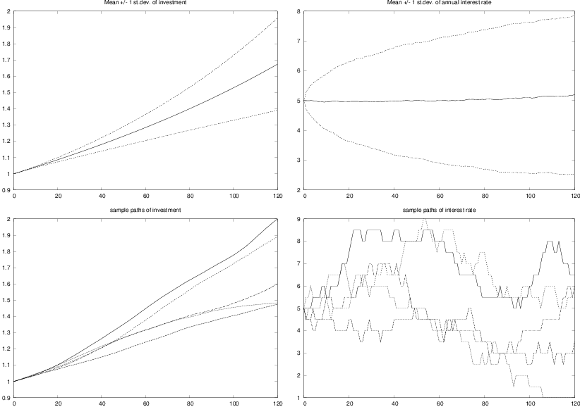
and initializing the seed of the random generator to 1, we get four plots, which are shown in Figure 8.
Figure 8: Development of an investment with random jumps of the interest rate at random points of time. Top left: mean value of investment \( \pm \) one standard deviation. Top right: mean value of the interest rate \( \pm \) one standard deviation. Bottom left: five paths of the investment development. Bottom right: five paths of the interest rate development.