This chapter is taken from the book A Primer on Scientific Programming with Python by H. P. Langtangen, 5th edition, Springer, 2016.
Random walk in one space dimension
In this section we shall simulate a collection of particles that move around in a random fashion. This type of simulations are fundamental in physics, biology, chemistry as well as other sciences and can be used to describe many phenomena. Some application areas include molecular motion, heat conduction, quantum mechanics, polymer chains, population genetics, brain research, hazard games, and pricing of financial instruments.
Imagine that we have some particles that perform random moves, either to the right or to the left. We may flip a coin to decide the movement of each particle, say head implies movement to the right and tail means movement to the left. Each move is one unit length. Physicists use the term random walk for this type of movement of a particle. You may try this yourself: flip the coin and make one step to the left or right, and repeat this process.
The movement is also known as drunkard's walk. You may have experienced this after a very wet night on a pub: you step forward and backward in a random fashion. Since these movements on average make you stand still, and since you know that you normally reach home within reasonable time, the model is not good for a real walk. We need to add a drift to the walk, so the probability is greater for going forward than backward. This is an easy adjustment, see Exercise 32: 1D random walk with drift. What may come as a surprise is the following fact: even when there is equal probability of going forward and backward, one can prove mathematically that the drunkard will always reach his home. Or more precisely, he will get home in finite time ("almost surely" as the mathematicians must add to this statement). Exercise 33: 1D random walk until a point is hit asks you to experiment with this fact. For many practical purposes, "finite time" does not help much as there might be more steps involved than the time it takes to get sufficiently sober to remove the completely random component of the walk.
Basic implementation
How can we implement \( n_s \) random steps of \( n_p \) particles in a program? Let us introduce a coordinate system where all movements are along the \( x \) axis. An array of \( x \) values then holds the positions of all particles. We draw random numbers to simulate flipping a coin, say we draw from the integers 1 and 2, where 1 means head (movement to the right) and 2 means tail (movement to the left). We think the algorithm is conveniently expressed directly as a complete Python program:
import random
import numpy
np = 4                          # no of particles
ns = 100                        # no of steps
positions = numpy.zeros(np)     # all particles start at x=0
HEAD = 1;  TAIL = 2             # constants

for step in range(ns):
    for p in range(np):
        coin = random.randint(1,2)  # flip coin
        if coin == HEAD:
            positions[p] += 1   # one unit length to the right
        elif coin == TAIL:
            positions[p] -= 1   # one unit length to the left
This program is found in the file walk1D.py.
Visualization
We may add some visualization of the movements by inserting a plot
command at the end of the step loop and a little pause to better
separate the frames in the animation:
    plot(positions, y, 'ko3', axis=[xmin, xmax, -0.2, 0.2])
    time.sleep(0.2)  # pause
These two statements require from scitools.std import plot and
import time.
It is very important that the extent of the axis are kept fixed in
animations, otherwise one gets a wrong visual impression. We know
that in \( n_s \) steps, no particle can move longer than \( n_s \) unit
lengths to the right or to the left so the extent of the \( x \) axis
becomes \( [-n_s,n_s] \). However, the probability of reaching these lower
or upper limit is very small. To be specific, the probability is
\( 2^{-n_s} \), which becomes about \( 10^{-9} \) for 30 steps. Most of the
movements will take place in the center of the plot. We may therefore
shrink the extent of the axis to better view the movements. It is
known that the expected extent of the particles is of the order
\( \sqrt{n_s} \), so we may take the maximum and minimum values in the
plot as \( \pm 2\sqrt{n_s} \). However, if a position of a particle
exceeds these values, we extend xmax and xmin by
\( 2\sqrt{n_s} \) in positive and negative \( x \) direction, respectively.
The \( y \) positions of the particles are taken as zero, but it is
necessary to have some extent of the \( y \) axis, otherwise the
coordinate system collapses and most plotting packages will refuse to
draw the plot. Here we have just chosen the \( y \) axis to go from -0.2
to 0.2. You can find the complete program in
walk1Dp.py. The np
and ns parameters can be set as the first two command-line
arguments:
walk1Dp.py 6 200
It is hard to claim that this program has astonishing graphics. In the section Random walk in two space dimensions, where we let the particles move in two space dimensions, the graphics gets much more exciting.
Random walk as a difference equation
The random walk process can easily be expressed in terms of a difference equation (see the document Sequences and difference equations [3] for an introduction to difference equations). Let \( x_n \) be the position of the particle at time \( n \). This position is an evolution from time \( n-1 \), obtained by adding a random variable \( s \) to the previous position \( x_{n-1} \), where \( s=1 \) has probability 1/2 and \( s=-1 \) has probability 1/2. In statistics, the expression probability of event A is written \( \Prob{A} \). We can therefore write \( \Prob{s=1}=1/2 \) and \( \Prob{s=-1}=1/2 \). The difference equation can now be expressed mathematically as $$ \begin{equation} x_n = x_{n-1} + s, \quad x_0=0,\quad {\rm P}(s=1)={\rm P}(s=-1)=1/2\tp \tag{10} \end{equation} $$ This equation governs the motion of one particle. For a collection \( m \) of particles we introduce \( x^{(i)}_n \) as the position of the \( i \)-th particle at the \( n \)-th time step. Each \( x^{(i)}_n \) is governed by (10), and all the \( s \) values in each of the \( m \) difference equations are independent of each other.
Computing statistics of the particle positions
Scientists interested in random walks are in general not interested in
the graphics of our walk1D.py program, but more in the
statistics of the positions of the particles at each step. We may
therefore, at each step, compute a histogram of the distribution of
the particles along the \( x \) axis, plus estimate the mean position and
the standard deviation. These mathematical operations are easily
accomplished by letting the SciTools function
compute_histogram and the numpy
functions mean and std operate on the positions
array (see the section Computing the mean and standard deviation)
:
    mean_pos  = numpy.mean(positions)
    stdev_pos = numpy.std(positions)
    pos, freq = compute_histogram(positions, nbins=int(xmax),
                                  piecewise_constant=True)
The number of bins in the histogram is just based on the extent of the particles. It could also have been a fixed number.
We can plot the particles as circles, as before, and add the histogram and vertical lines for the mean and the positive and negative standard deviation (the latter indicates the "width" of the distribution of particles). The vertical lines can be defined by the six lists
    xmean, ymean   = [mean_pos, mean_pos],     [yminv, ymaxv]
    xstdv1, ystdv1 = [stdev_pos, stdev_pos],   [yminv, ymaxv]
    xstdv2, ystdv2 = [-stdev_pos, -stdev_pos], [yminv, ymaxv]
where yminv and ymaxv are the minimum and maximum
\( y \) values of the vertical lines.
The following command plots the position of every particle
as circles, the histogram as a curve,
and the vertical lines with a thicker line:
    plot(positions, y, 'ko3',     # particles as circles
         pos, freq, 'r',          # histogram
         xmean, ymean, 'r2',      # mean position as thick line
         xstdv1, ystdv1, 'b2',    # +1 standard dev.
         xstdv2, ystdv2, 'b2',    # -1 standard dev.
         axis=[xmin, xmax, ymin, ymax],
         title='random walk of %d particles after %d steps' %
               (np, step+1))
This plot is then created at every step in the random walk. By
observing the graphics, one will soon realize that the computation of
the extent of the \( y \) axis in the plot needs some considerations. We
have found it convenient to base ymax on the maximum value of the
histogram (max(freq)), plus some space (chosen as 10 percent of
max(freq)). However, we do not change the ymax value unless it is
more than 0.1 different from the previous ymax value (otherwise the
axis "jumps" too often). The minimum value, ymin, is set to
ymin=-0.1*ymax every time we change the ymax value. The complete
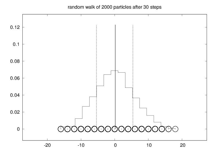
code is found in the file walk1Ds.py. If you try out 2000 particles and 30
steps, the final graphics becomes like that in Figure
6. As the number of steps is increased, the
particles are dispersed in the positive and negative \( x \) direction,
and the histogram gets flatter and flatter. Letting \( \hat H(i) \) be the
histogram value in interval number \( i \), and each interval having width
\( \Delta x \), the probability of finding a particle in interval \( i \) is
\( \hat H(i)\Delta x \). It can be shown mathematically that the
histogram is an approximation to the probability density function of
the normal distribution with mean zero and standard deviation \( s\sim
\sqrt{n} \), where \( n \) is the step number.
Figure 6: Particle positions (circles), histogram (piecewise constant curve), and vertical lines indicating the mean value and the standard deviation from the mean after a one-dimensional random walk of 2000 particles for 30 steps.
Vectorized implementation
There is no problem with the speed of our one-dimensional random walkers
in the walk1Dp.py or walk1Ds.py programs,
but in real-life applications of such
simulation models, we often have a very large number of particles performing
a very large number of steps. It is then important to make the implementation
as efficient as possible. Two loops over all particles and all steps,
as we have in the programs above, become
very slow compared to a vectorized implementation.
A vectorized implementation of a one-dimensional walk should utilize
the functions randint
or random_integers from numpy's random module. A first idea may be to
draw steps for all particles at a step simultaneously. Then we repeat
this process in a loop from 0 to \( n_s-1 \). However, these repetitions
are just new vectors of random numbers, and we may avoid the loop
if we draw \( n_p\times n_s \) random numbers at once:
moves = numpy.random.randint(1, 3, size=np*ns)
# or
moves = numpy.random.random_integers(1, 2, size=np*ns)
The values are now either 1 or 2, but we want \( -1 \) or \( 1 \). A simple scaling and translation of the numbers transform the 1 and 2 values to \( -1 \) and \( 1 \) values:
moves = 2*moves - 3
Then we can create a two-dimensional array out of moves such
that moves[i,j] is the i-th step of particle number j:
moves.shape = (ns, np)
It does not make sense to plot the evolution of the particles and the
histogram in the vectorized version of the code, because the point with
vectorization is to speed up the calculations, and the visualization
takes much more time than drawing random numbers, even in the
walk1Dp.py and walk1Ds.py programs from
the section Computing statistics of the particle positions. We therefore just
compute the positions of the particles inside a loop over the steps
and some simple statistics. At the end, after \( n_s \) steps, we
plot the histogram of the particle distribution along with circles for
the positions of the particles. The rest of the program, found in
the file walk1Dv.py, looks as follows:
positions = numpy.zeros(np)
for step in range(ns):
    positions += moves[step, :]

    mean_pos = numpy.mean(positions)
    stdev_pos = numpy.std(positions)
    print mean_pos, stdev_pos

nbins = int(3*sqrt(ns))    # no of intervals in histogram
pos, freq = compute_histogram(positions, nbins,
                              piecewise_constant=True)

plot(positions, zeros(np), 'ko3',
     pos, freq, 'r',
     axis=[min(positions), max(positions), -0.01, 1.1*max(freq)],
     savefig='tmp.pdf')