This chapter is taken from the book A Primer on Scientific Programming with Python by H. P. Langtangen, 5th edition, Springer, 2016.
Simple games
This section presents the implementation of some simple games based on drawing random numbers. The games can be played by two humans, but here we consider a human versus the computer.
Guessing a number
The game
The computer determines a secret number, and the player shall guess the number. For each guess, the computer tells if the number is too high or too low.
The implementation
We let the computer draw a random integer in an interval known to the
player, let us say \( [1,100] \).
In a while loop the program prompts the player for a guess,
reads the guess, and checks if the guess is higher or lower than the
drawn number. An appropriate message is written to the screen.
We think the algorithm can be expressed directly as executable Python code:
import random
number = random.randint(1, 100)
attempts = 0  # count no of attempts to guess the number
guess = 0
while guess != number:
    guess = eval(raw_input('Guess a number: '))
    attempts += 1
    if guess == number:
        print 'Correct! You used', attempts, 'attempts!'
        break
    elif guess < number:
        print 'Go higher!'
    else:
        print 'Go lower!'
The program is available as the file guess_number.py. Try it out! Can you come up with a strategy for reducing the number of attempts? See Exercise 27: Investigate guessing strategies for an automatic investigation of two possible strategies.
Rolling two dice
The game
The player is supposed to roll two dice, and beforehand guess the sum of the eyes. If the guess on the sum is \( n \) and it turns out to be right, the player earns \( n \) euros. Otherwise, the player must pay 1 euro. The machine plays in the same way, but the machine's guess of the number of eyes is a uniformly distributed number between 2 and 12. The player determines the number of rounds, \( r \), to play, and receives \( r \) euros as initial capital. The winner is the one that has the largest amount of euros after \( r \) rounds, or the one that avoids to lose all the money.
The implementation
There are three actions that we can naturally implement as functions:
(i) roll two dice and compute the sum; (ii) ask the player to guess
the number of eyes; (iii) draw the computer's guess of the number of
eyes. One soon realizes that it is as easy to implement this game
for an arbitrary number of dice as it is for two dice. Consequently we can
introduce ndice as the number of dice.
The three functions take the following forms:
import random

def roll_dice_and_compute_sum(ndice):
    return sum([random.randint(1, 6) \
                for i in range(ndice)])

def computer_guess(ndice):
    return random.randint(ndice, 6*ndice)

def player_guess(ndice):
    return input('Guess the sum of the no of eyes '\
                 'in the next throw: ')
We can now implement one round in the game for the player or the computer. The round starts with a capital, a guess is performed by calling the right function for guessing, and the capital is updated:
def play_one_round(ndice, capital, guess_function):
    guess = guess_function(ndice)
    throw = roll_dice_and_compute_sum(ndice)
    if guess == throw:
        capital += guess
    else:
        capital -= 1
    return capital, throw, guess
Here, guess_function is either
computer_guess or
player_guess.
With the play_one_round function we can run a number of rounds
involving both players:
def play(nrounds, ndice=2):
    player_capital = computer_capital = nrounds  # start capital

    for i in range(nrounds):
        player_capital, throw, guess = \
             play_one_round(ndice, player_capital, player_guess)
        print 'YOU guessed %d, got %d' % (guess, throw)

        computer_capital, throw, guess = \
            play_one_round(ndice, computer_capital, computer_guess)

        print 'Machine guessed %d, got %d' % (guess, throw)

        print 'Status: you have %d euros, machine has %d euros' % \
              (player_capital, computer_capital)

        if player_capital == 0 or computer_capital == 0:
            break

    if computer_capital > player_capital:
        winner = 'Machine'
    else:
        winner = 'You'
    print winner, 'won!'
The name of the program is ndice.py.
Example
Here is a session (with a fixed seed of 20):
Guess the sum of the no of eyes in the next throw: 7
YOU guessed 7, got 11
Machine guessed 10, got 8
Status: you have 9 euros, machine has 9 euros

Guess the sum of the no of eyes in the next throw: 9
YOU guessed 9, got 10
Machine guessed 11, got 6
Status: you have 8 euros, machine has 8 euros

Guess the sum of the no of eyes in the next throw: 9
YOU guessed 9, got 9
Machine guessed 3, got 8
Status: you have 17 euros, machine has 7 euros
Exercise 12: Compare two playing strategies asks you to perform simulations to determine whether a certain strategy can make the player win over the computer in the long run.
A class version
We can cast the previous code segment in a class. Many will argue that a class-based implementation is closer to the problem being modeled and hence easier to modify or extend.
A natural class is Dice,
which can throw n dice:
class Dice(object):
    def __init__(self, n=1):
        self.n = n   # no of dice

    def throw(self):
        return [random.randint(1,6) \
                for i in range(self.n)]
Another natural class is Player, which can perform
the actions of a player.
Functions can then make use of Player to set up a game.
A Player has a name, an initial capital, a set of dice,
and a Dice object to throw the object:
class Player(object):
    def __init__(self, name, capital, guess_function, ndice):
        self.name = name
        self.capital = capital
        self.guess_function = guess_function
        self.dice = Dice(ndice)

    def play_one_round(self):
        self.guess = self.guess_function(self.dice.n)
        self.throw = sum(self.dice.throw())
        if self.guess == self.throw:
            self.capital += self.guess
        else:
            self.capital -= 1
        self.message()
        self.broke()

    def message(self):
        print '%s guessed %d, got %d' % \
              (self.name, self.guess, self.throw)

    def broke(self):
        if self.capital == 0:
            print '%s lost!' % self.name
            sys.exit(0)  # end the program
The guesses of the computer and the player are specified by functions:
def computer_guess(ndice):
    # All guesses have the same probability
    return random.randint(ndice, 6*ndice)

def player_guess(ndice):
    return input('Guess the sum of the no of eyes '\
                 'in the next throw: ')
The key function to play the whole game, utilizing the Player class
for the computer and the user,
can be expressed as
def play(nrounds, ndice=2):
    player = Player('YOU', nrounds, player_guess, ndice)
    computer = Player('Computer', nrounds, computer_guess, ndice)

    for i in range(nrounds):
        player.play_one_round()
        computer.play_one_round()
        print 'Status: user has %d euro, machine has %d euro\n' % \
              (player.capital, computer.capital)

    if computer.capital > player.capital:
        winner = 'Machine'
    else:
        winner = 'You'
    print winner, 'won!'
The complete code is found in the file ndice2.py. There is no new functionality compared
to the ndice.py implementation, just a new and better structuring of
the code.
Monte Carlo integration
One of the earliest applications of random numbers was numerical computation of integrals, which is actually non-random (deterministic) problem. Computing integrals with the aid of random numbers is known as Monte Carlo integration and is one of the most powerful and widely used mathematical technique throughout science and engineering.
Our main focus here will be integrals of the type \( \int_a^b f(x)dx \) for which the Monte Carlo integration is not a competitive technique compared to simple methods such as the Trapezoidal method, the Midpoint method, or Simpson's method. However, for integration of functions of many variables, the Monte Carlo approach is the best method we have. Such integrals arise all the time in quantum physics, financial engineering, and when estimating the uncertainty of mathematical computations. What you learn about Monte Carlo integration of functions of one variable (\( \int_a^b f(x)dx \)) is directly transferable to the important application cases where there are many variables involved.
Derivation of Monte Carlo integration
There are two ways to introduce Monte Carlo integration, one based on calculus and one based on probability theory. The goal is to compute a numerical approximation to $$ \int_a^b f(x)dx\tp$$
The calculus approach via the mean-value theorem
The mean-value theorem from calculus states that $$ \begin{equation} \int_a^b f(x)dx = (b-a)\bar f, \tag{7} \end{equation} $$ where \( \bar f \) is the mean value of \( f \), defined as $$ \bar f = {1\over b-a}\int_a^b f(x)dx\tp $$ One way of using (7) to define a numerical method for integration is to approximate \( \bar f \) by taking the average of \( f \) at \( n \) points \( x_0,\ldots,x_{n-1} \): $$ \begin{equation} \bar f\approx \frac{1}{n}\sum_{i=0}^{n-1} f(x_i)\tp \tag{8} \end{equation} $$ (We let the numbering of the points go from \( 0 \) to \( n-1 \) because these numbers will later be indices in Python arrays, which have to start at \( 0 \).)
There is freedom in how to choose the points \( x_0,\ldots,x_{n-1} \). We could, for example, make them uniformly spaced in the interval \( [a, b] \). The particular choice $$ x_0 = a + ih + \frac{1}{2}h,\quad i=0,\ldots,n-1,\quad h=\frac{b-a}{n-1},$$ correspond to the famous Midpoint rule for numerical integration. Intuitively, we anticipate that the more points we use, the better is the approximation \( \frac{1}{n}\sum_if(x_i) \) to the exact mean value \( \bar f \). For the Midpoint rule one can show mathematically, or numerically estimate through examples, that the error in the approximation depends on \( n \) as \( n^{-2} \). That is, doubling the number of points reduces the error by a factor 1/4.
A slightly different set of uniformly distributed points is $$ x_i = a + ih,\quad i=0,\ldots,n-1,\ldots,\quad h=\frac{b-1}{n-2}\tp$$ These points might look more intuitive to many since they start at \( a \) and end at \( b \) (\( x_0=a \), \( x_{n-1}=b \)), but the error in the integration rule now goes as \( n^{-1} \): doubling the number of points just halves the error. That is, computing more function values to get a better integration estimate is less effective with this set points than with the slight displaced points used in the Midpoint rule.
One could also throw in the idea of using a set of random points, uniformly distributed in \( [a,b] \). This is the Monte Carlo integration technique. The error now goes like \( n^{-1/2} \), which means that many more points and corresponding function evaluations are needed to reduce the error compared to using the Midpoint method. The surprising fact, however, is that using random points for many variables (in high-dimensional vector spaces) yields a very effective integration technique, dramatically more effective than extending the ideas of the Midpoint rule to many variables.
The probability theory approach
People who are into probability theory usually like to interpret integrals as mathematical expectations of a random variable. (If you are not one of those, you can safely jump to the section Implementation of standard Monte Carlo integration where we just program the simple sum in the Monte Carlo integration method.) More precisely, the integral \( \int_a^b f(x)dx \) can be expressed as a mathematical expectation of \( f(x) \) if \( x \) is a uniformly distributed random variable on \( [a,b] \). This expectation can be estimated by the average of random samples, which results in the Monte Carlo integration method. To see this, we start with the formula for the probability density function for a uniformly distributed random variable \( X \) on \( [a,b] \): $$ p(x) =\left\lbrace\begin{array}{ll} (b-a)^{-1},& x\in [a,b]\\ 0, & \hbox{otherwise} \end{array}\right. $$ Now we can write the standard formula for the mathematical expectation \( \mbox{E}(f(X)) \): $$ \mbox{E}(f(X)) = \int_{-\infty}^{\infty} f(x)p(x)dx = \int_a^b f(x)\frac{1}{b-a}dx = (b-a)\int_a^b f(x)dx\tp $$ The last integral is exactly what we want to compute. An expectation is usually estimated from a lot of samples, in this case uniformly distributed random numbers \( x_0,\ldots,x_{n-1} \) in \( [a,b] \), and computing the sample mean: $$ \mbox{E}(f(X)) \approx \frac{1}{n}\sum_{i=0}^{n-1} f(x_i)\tp$$ The integral can therefore be estimated by $$ \int_a^b f(x)dx\approx (b-a)\frac{1}{n}\sum_{i=0}^{n-1} f(x_i),$$ which is nothing but the Monte Carlo integration method.
Implementation of standard Monte Carlo integration
To summarize, Monte Carlo integration consists in generating \( n \) uniformly distributed random numbers \( x_i \) in \( [a,b] \) and then compute $$ \begin{equation} (b-a)\frac{1}{n}\sum_{i=0}^{n-1} f(x_i)\tp \tag{9} \end{equation} $$ We can implement (9) in a small function:
import random

def MCint(f, a, b, n):
    s = 0
    for i in xrange(n):
        x = random.uniform(a, b)
        s += f(x)
    I = (float(b-a)/n)*s
    return I
One normally needs a large \( n \) to obtain good results with this method,
so a faster vectorized version of the MCint function is very useful:
import numpy as np

def MCint_vec(f, a, b, n):
    x = np.random.uniform(a, b, n)
    s = np.sum(f(x))
    I = (float(b-a)/n)*s
    return I
The functions above are available in the module
file MCint.py.
We can test the gain in efficiency with %timeit in an IPython session:
In [1]: from MCint import MCint, MCint_vec

In [2]: from math import sin, pi

In [3]: %timeit MCint(sin, 0, pi, 1000000)
1 loops, best of 3: 1.19 s per loop

In [4]: from numpy import sin

In [5]: %timeit MCint_vec(sin, 0, pi, 1000000)
1 loops, best of 3: 173 ms per loop

In [6]: 1.19/0.173          # relative performance
Out[6]: 6.878612716763006
Note that we use sin from math in the scalar function MCint
because this function is significantly faster than sin from
numpy:
In [7]: from math import sin

In [8]: %timeit sin(1.2)
10000000 loops, best of 3: 179 ns per loop

In [9]: from numpy import sin

In [10]: %timeit sin(1.2)
100000 loops, best of 3: 3.22 microsec per loop

In [11]: 3.22E-6/179E-9      # relative performance
Out[11]: 17.988826815642458
(A similar test reveals that math.sin is 1.3 times slower calling
sin without a prefix. The differences are much smaller between
numpy.sin and the same function without the prefix.)
The increase in efficiency by using MCint_vec instead of
MCint is in the test above a factor of 6-7, which is not dramatic.
Moreover, the vectorized version needs to store \( n \) random numbers
and \( n \) function values
in memory. A better vectorized implementation for large \( n \)
is to split the x and f(x) arrays into chunks of a given size
arraysize such that we can control the memory usage.
Mathematically, it means to split the sum \( \frac{1}{n}\sum_i f(x_i) \)
into a sum of smaller sums. An appropriate implementation reads
def MCint_vec2(f, a, b, n, arraysize=1000000):
    s = 0
    # Split sum into batches of size arraysize
    # + a sum of size rest (note: n//arraysize is integer division)
    rest = n % arraysize
    batch_sizes = [arraysize]*(n//arraysize) + [rest]
    for batch_size in batch_sizes:
        x = np.random.uniform(a, b, batch_size)
        s += np.sum(f(x))
    I = (float(b-a)/n)*s
    return I
With 100 million points, MCint_vec2 is about 10 faster than MCint.
(Note that the latter function must use xrange and not range
for so large \( n \), otherwise the array returned by range may become
to large to be stored in memory in a small computer. The xrange
function generates one i at a time without the need to store all
the i values.)
Example
Let us try the Monte Carlo integration method on a simple linear function \( f(x)=2+3x \), integrated from 1 to 2. Most other numerical integration methods will integrate such a linear function exactly, regardless of the number of function evaluations. This is not the case with Monte Carlo integration.
It would be interesting to see how the quality of the
Monte Carlo approximation increases with \( n \).
To plot the evolution of the integral approximation we must store
intermediate I values. This requires a slightly
modified MCint method:
def MCint2(f, a, b, n):
    s = 0
    # Store the intermediate integral approximations in an
    # array I, where I[k-1] corresponds to k function evals.
    I = np.zeros(n)
    for k in range(1, n+1):
        x = random.uniform(a, b)
        s += f(x)
        I[k-1] = (float(b-a)/k)*s
    return I
Note that we let k go from 1 to n, such that k reflects the
actual number of points used in the method. Since n can be very
large, the I array may consume more memory than what we have
on the computer. Therefore, we decide to store only
every \( N \) values of the approximation. Determining if a value is to be stored
or not can be computed by
the mod function: k % N gives the remainder when k is
divided by N. In our case we can store when this reminder is zero,
for k in range(1, n+1):
    ...
    if k % N == 0:
        # store
This recipe of doing something every \( N \)-th pass in long loops has lots of applications in scientific computing! The complete function now takes the following form:
def MCint3(f, a, b, n, N=100):
    s = 0
    # Store every N intermediate integral approximations in an
    # array I and record the corresponding k value.
    I_values = []
    k_values = []
    for k in range(1, n+1):
        x = random.uniform(a, b)
        s += f(x)
        if k % N == 0:
            I = (float(b-a)/k)*s
            I_values.append(I)
            k_values.append(k)
    return k_values, I_values

def demo():
Our sample application goes like
def f1(x):
    return 2 + 3*x

k, I = MCint3(f1, 1, 2, 1000000, N=10000)
error = 6.5 - np.array(I)
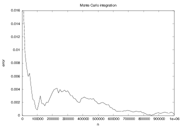
Figure 4 shows a plot of error versus the
number of function evaluation k.
Figure 4: The convergence of Monte Carlo integration applied to \( \int_1^2 (2 + 3x)dx \).
Remark
We claimed that the Monte Carlo method is slow for integration functions of one variable. There are, however, many techniques that apply smarter ways of drawing random numbers, so called variance reduction techniques, and thereby increase the computational efficiency.
Area computing by throwing random points
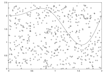
Think of some geometric region \( G \) in the plane and a surrounding bounding box \( B \) with geometry \( [x_L,x_H]\times[y_L,y_H] \). One way of computing the area of \( G \) is to draw \( N \) random points inside \( B \) and count how many of them, \( M \), that lie inside \( G \). The area of \( G \) is then the fraction \( M/N \) (\( G \)'s fraction of \( B \)'s area) times the area of \( B \), \( (x_H-x_L)(y_H-y_L) \). Phrased differently, this method is a kind of dart game where you record how many hits there are inside \( G \) if every throw hits uniformly within \( B \).
Let us formulate this method for computing the integral \( \int_a^bf(x)dx \). The important observation is that this integral is the area under the curve \( y=f(x) \) and above the \( x \) axis, between \( x=a \) and \( x=b \). We introduce a rectangle \( B \), $$ \begin{equation*} B = \{ (x,y)\, |\, a\leq x\leq b, \ 0\leq y\leq m \},\end{equation*} $$ where \( m\leq\max_{x\in [a,b]} f(x) \). The algorithm for computing the area under the curve is to draw \( N \) random points inside \( B \) and count how many of them, \( M \), that are above the \( x \) axis and below the \( y=f(x) \) curve, see Figure 5. The area or integral is then estimated by $$ \begin{equation*} \frac{M}{N}m(b-a)\tp\end{equation*} $$
Figure 5: The "dart" method for computing integrals. When \( M \) out of \( N \) random points in the rectangle \( [0,2]\times [0,2.4] \) lie under the curve, the area under the curve is estimated as the \( M/N \) fraction of the area of the rectangle, i.e., \( (M/N) 2\cdot 2.4 \).
First we implement the "dart method" by a simple loop over points:
def MCint_area(f, a, b, n, m):
    below = 0  # counter for no of points below the curve
    for i in range(n):
        x = random.uniform(a, b)
        y = random.uniform(0, m)
        if y <= f(x):
            below += 1
    area = below/float(n)*m*(b-a)
    return area
Note that this method draws twice as many random numbers as the previous method.
A vectorized implementation reads
import numpy as np

def MCint_area_vec(f, a, b, n, m):
    x = np.random.uniform(a, b, n)
    y = np.random.uniform(0, m, n)
    below = np.sum(y < f(x))
    area = below/float(n)*m*(b-a)
    return area
The only non-trivial line here is the expression y[y < f(x)],
which applies boolean indexing
to extract the y values that are below the f(x) curve.
The sum of the boolean values (interpreted as 0 and 1)
in y < f(x) gives the number of points below the curve.
Even for 2 million random numbers the plain loop version is not that
slow as it executes within some seconds on a slow laptop.
Nevertheless,
if you need the integration being repeated many times
inside another calculation, the superior efficiency of
the vectorized version may be important. We can quantify the
efficiency gain by the aid of the timer time.clock() in the
following
way:
import time
t0 = time.clock()
print MCint_area(f1, a, b, n, fmax)
t1 = time.clock()   # time of MCint_area is t1-t0
print MCint_area_vec(f1, a, b, n, fmax)
t2 = time.clock()   # time of MCint_area_vec is t2-t1
print 'loop/vectorized fraction:', (t1-t0)/(t2-t1)
With \( n=10^6 \) the author achieved a factor of about 8 in favor of the vectorized version.