This chapter is taken from the book A Primer on Scientific Programming with Python by H. P. Langtangen, 5th edition, Springer, 2016.
Random walk in two space dimensions
A random walk in two dimensions performs a step either to the north, south, west, or east, each one with probability \( 1/4 \). To demonstrate this process, we introduce \( x \) and \( y \) coordinates of \( n_p \) particles and draw random numbers among 1, 2, 3, or 4 to determine the move. The positions of the particles can easily be visualized as small circles in an \( xy \) coordinate system.
Basic implementation
The algorithm described above is conveniently expressed directly as a complete working program:
def random_walk_2D(np, ns, plot_step):
    xpositions = numpy.zeros(np)
    ypositions = numpy.zeros(np)
    # extent of the axis in the plot:
    xymax = 3*numpy.sqrt(ns); xymin = -xymax

    NORTH = 1;  SOUTH = 2;  WEST = 3;  EAST = 4  # constants

    for step in range(ns):
        for i in range(np):
            direction = random.randint(1, 4)
            if direction == NORTH:
                ypositions[i] += 1
            elif direction == SOUTH:
                ypositions[i] -= 1
            elif direction == EAST:
                xpositions[i] += 1
            elif direction == WEST:
                xpositions[i] -= 1

        # Plot just every plot_step steps
        if (step+1) % plot_step == 0:
            plot(xpositions, ypositions, 'ko',
                 axis=[xymin, xymax, xymin, xymax],
                 title='%d particles after %d steps' %
                       (np, step+1),
                 savefig='tmp_%03d.pdf' % (step+1))
    return xpositions, ypositions

# main program:
import random
random.seed(10)
import sys
import numpy
from scitools.std import plot

np        = int(sys.argv[1])  # number of particles
ns        = int(sys.argv[2])  # number of steps
plot_step = int(sys.argv[3])  # plot every plot_step steps
x, y = random_walk_2D(np, ns, plot_step)
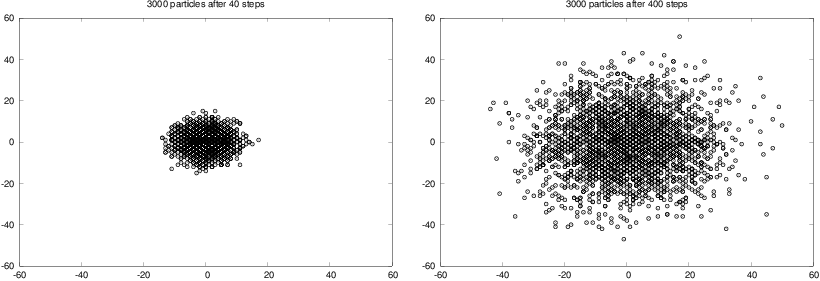
The program is found in the file walk2D.py. Figure
7 shows two snapshots of the
distribution of 3000 particles after 40 and 400 steps. These plots
were generated with command-line arguments 3000 400 20, the latter
implying that we visualize the particles every 20 time steps only.
Figure 7: Location of 3000 particles starting at the origin and performing a random walk, with 40 steps (left) and 400 steps (right).
To get a feeling for the two-dimensional random walk you can try out
only 30 particles for 400 steps and let each step be visualized
(i.e., command-line arguments 30 400 1).
The update of the movements is now fast.
The walk2D.py program dumps the plots to PDF files
with names of the form tmp_xxx.pdf, where xxx is
the step number. We can create a movie out of these individual
files using the program convert from the ImageMagick suite:
Terminal> convert -delay 50 -loop 1000 tmp_*.pdf movie.gif
All the plots are now put after each other as frames in a movie, with
a delay of 50 ms between each frame. The movie will run in a loop
1000 times.
The resulting movie file is named movie.gif, which can
be viewed by the animate program (also from the ImageMagick
program suite), just write animate movie.gif.
Making and showing the movie are slow processes if a large number of
steps are included in the movie. The alternative is to make
a true video file in, e.g., the Flash format:
Terminal> avconv -r 5 -i tmp_%04d.png -c:v flv movie.flv
This requires the plot files to be in PNG format.
Vectorized implementation
The walk2D.py program is quite slow. Now the visualization is much
faster than the movement of the particles. Vectorization may speed up
the walk2D.py program significantly. As in the one-dimensional
phase, we draw all the movements at once and then invoke a loop over
the steps to update the \( x \) and \( y \) coordinates. We draw \( n_s\times
n_p \) numbers among 1, 2, 3, and 4. We then reshape the vector of
random numbers to a two-dimensional array moves[i, j], where i
counts the steps, j counts the particles. The if test on whether
the current move is to the north, south, east, or west can be
vectorized using the where
function.
For example, if the random numbers for all particles in the current step
are accessible in an array this_move, we could update the \( x \)
positions by
xpositions += np.where(this_move == EAST, 1, 0)
xpositions -= np.where(this_move == WEST, 1, 0)
provided EAST and WEST are constants, equal to 3 and 4,
respectively. A similar construction can be used for the \( y \) moves.
The complete program is listed below:
def random_walk_2D(np, ns, plot_step):
    xpositions = numpy.zeros(np)
    ypositions = numpy.zeros(np)
    moves = numpy.random.random_integers(1, 4, size=ns*np)
    moves.shape = (ns, np)

    # Estimate max and min positions
    xymax = 3*numpy.sqrt(ns); xymin = -xymax

    NORTH = 1;  SOUTH = 2;  WEST = 3;  EAST = 4  # constants

    for step in range(ns):
        this_move = moves[step,:]
        ypositions += numpy.where(this_move == NORTH, 1, 0)
        ypositions -= numpy.where(this_move == SOUTH, 1, 0)
        xpositions += numpy.where(this_move == EAST,  1, 0)
        xpositions -= numpy.where(this_move == WEST,  1, 0)

        # Just plot every plot_step steps
        if (step+1) % plot_step == 0:
            plot(xpositions, ypositions, 'ko',
                 axis=[xymin, xymax, xymin, xymax],
                 title='%d particles after %d steps' %
                       (np, step+1),
                 savefig='tmp_%03d.pdf' % (step+1))
    return xpositions, ypositions

# Main program
from scitools.std import plot
import numpy, sys
numpy.random.seed(11)

np = int(sys.argv[1])  # number of particles
ns = int(sys.argv[2])  # number of steps
plot_step = int(sys.argv[3])  # plot each plot_step step
x, y = random_walk_2D(np, ns, plot_step)
You will easily experience that this program, found in the file
walk2Dv.py, runs significantly
faster than the walk2D.py program.