This chapter is taken from the book A Primer on Scientific Programming with Python by H. P. Langtangen, 5th edition, Springer, 2016.

Drawing random numbers

Python has a module random for generating random numbers. The function call random.random() generates a random number in the half open interval \( [0, 1) \) (recall that in the half open interval \( [0,1) \) the lower limit is included, but the upper limit is not). We can try it out:

>>> import random
>>> random.random()
0.81550546885338104
>>> random.random()
0.44913326809029852
>>> random.random()
0.88320653116367454

All computations of random numbers are based on deterministic algorithms (see Exercise 20: Difference equation for random numbers for an example), so the sequence of numbers cannot be truly random. However, the sequence of numbers appears to lack any pattern, and we can therefore view the numbers as random.

The seed

Every time we import random, the subsequent sequence of random.random() calls will yield different numbers. For debugging purposes it is useful to get the same sequence of random numbers every time we run the program. This functionality is obtained by setting a seed before we start generating numbers. With a given value of the seed, one and only one sequence of numbers is generated. The seed is an integer and set by the random.seed function:

>>> random.seed(121)

Let us generate two series of random numbers at once, using a list comprehension and a format with two decimals only:

>>> random.seed(2)
>>> ['%.2f' % random.random() for i in range(7)]
['0.96', '0.95', '0.06', '0.08', '0.84', '0.74', '0.67']
>>> ['%.2f' % random.random() for i in range(7)]
['0.31', '0.61', '0.61', '0.58', '0.16', '0.43', '0.39']

If we set the seed to 2 again, the sequence of numbers is regenerated:

>>> random.seed(2)
>>> ['%.2f' % random.random() for i in range(7)]
['0.96', '0.95', '0.06', '0.08', '0.84', '0.74', '0.67']

If we do not give a seed, the random module sets a seed based on the current time. That is, the seed will be different each time we run the program and consequently the sequence of random numbers will also be different from run to run. This is what we want in most applications. However, we always recommend setting a seed during program development to simplify debugging and verification.

Uniformly distributed random numbers

The numbers generated by random.random() tend to be equally distributed between 0 and 1, which means that there is no part of the interval \( [0,1) \) with more random numbers than other parts. We say that the distribution of random numbers in this case is uniform. The function random.uniform(a,b) generates uniform random numbers in the half open interval \( [a,b) \), where the user can specify \( a \) and \( b \). With the following program (in file uniform_numbers0.py) we may generate lots of random numbers in the interval \( [-1,1) \) and visualize how they are distributed :

import random
random.seed(42)
N = 500  # no of samples
x = range(N)
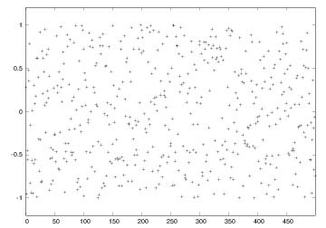
y = [random.uniform(-1,1) for i in x]

import scitools.std as st
st.plot(x, y, '+', axis=[0,N-1,-1.2,1.2])

Figure 1 shows the values of these 500 numbers, and as seen, the numbers appear to be random and uniformly distributed between \( -1 \) and \( 1 \).

Visualizing the distribution

It is of interest to see how \( N \) random numbers in an interval \( [a,b] \) are distributed throughout the interval, especially as \( N\rightarrow\infty \). For example, when drawing numbers from the uniform distribution, we expect that no parts of the interval get more numbers than others. To visualize the distribution, we can divide the interval into subintervals and display how many numbers there are in each subinterval.

Let us formulate this method more precisely. We divide the interval \( [a,b) \) into \( n \) equally sized subintervals, each of length \( h=(b-a)/n \). These subintervals are called bins. We can then draw \( N \) random numbers by calling random.random() \( N \) times. Let \( \hat H(i) \) be the number of random numbers that fall in bin no. \( i \), \( [a+ih, a+(i+1)h] \), \( i=0,\ldots,n-1 \). If \( N \) is small, the value of \( \hat H(i) \) can be quite different for the different bins, but as \( N \) grows, we expect that \( \hat H(i) \) varies little with \( i \).

Ideally, we would be interested in how the random numbers are distributed as \( N\rightarrow\infty \) and \( n\rightarrow\infty \). One major disadvantage is that \( \hat H(i) \) increases as \( N \) increases, and it decreases with \( n \). The quantity \( \hat H(i)/N \), called the frequency count, will reach a finite limit as \( N\rightarrow\infty \). However, \( \hat H(i)/N \) will be smaller and smaller as we increase the number of bins. The quantity \( H(i) = \hat H(i)/(Nh) \) reaches a finite limit as \( N,n\rightarrow\infty \). The probability that a random number lies inside subinterval no. \( i \) is then \( \hat H(i)/N = H(i)h \).

We can visualize \( H(i) \) as a bar diagram (see Figure 2), called a normalized histogram. We can also define a piecewise constant function \( p(x) \) from \( H(i) \): \( p(x) = H(i) \) for \( x\in [a+ih, a+(i+1)h) \), \( i=0,\ldots,n-1 \). As \( n,N\rightarrow\infty \), \( p(x) \) approaches the probability density function of the distribution in question. For example, random.uniform(a,b) draws numbers from the uniform distribution on \( [a,b) \), and the probability density function is constant, equal to \( 1/(b-a) \). As we increase \( n \) and \( N \), we therefore expect \( p(x) \) to approach the constant \( 1/(b-a) \).

The function compute_histogram from scitools.std returns two arrays x and y such that plot(x,y) plots the piecewise constant function \( p(x) \). The plot is hence the histogram of the set of random samples. The program below exemplifies the usage:

from scitools.std import plot, compute_histogram
import random
samples = [random.random() for i in range(100000)]
x, y = compute_histogram(samples, nbins=20)
plot(x, y)

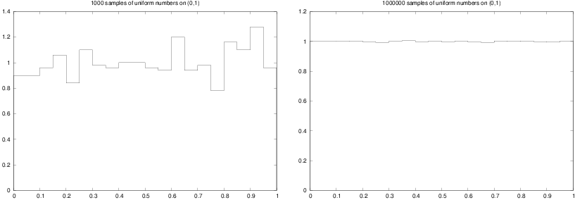
Figure 2 shows two plots corresponding to \( N \) taken as \( 10^3 \) and \( 10^6 \). For small \( N \), we see that some intervals get more random numbers than others, but as \( N \) grows, the distribution of the random numbers becomes more and more equal among the intervals. In the limit \( N\rightarrow\infty \), \( p(x)\rightarrow 1 \), which is illustrated by the plot.

Vectorized drawing of random numbers

There is a random module in the Numerical Python package, which can be used to efficiently draw a possibly large array of random numbers:

import numpy as np
r = np.random.random()            # one number between 0 and 1
r = np.random.random(size=10000)  # array with 10000 numbers
r = np.random.uniform(-1, 10)     # one number between -1 and 10
r = np.random.uniform(-1, 10, size=10000)  # array

There are thus two random modules to be aware of: one in the standard Python library and one in numpy. For drawing uniformly distributed numbers, the two random modules have the same interface, except that the functions from numpy's random module has an extra size parameter. Both modules also have a seed function for fixing the seed.

Vectorized drawing of random numbers using numpy's random module is efficient because all the numbers are drawn "at once" in fast C code. You can measure the efficiency gain with the time.clock() function.

Warning

It is easy to do an import random followed by a from numpy import * or maybe from scitools.std import * without realizing that the latter two import statements import a name random from numpy that overwrites the same name that was imported in import random. The result is that the effective random module becomes the one from numpy. A possible solution to this problem is to introduce a different name for Python's random module, say

import random as random_number

Another solution is to do import numpy as np and work explicitly with np.random.

Computing the mean and standard deviation

You probably know the formula for the mean or average of a set of \( n \) numbers \( x_0,x_1,\ldots,x_{n-1} \): $$ \begin{equation} x_m = \frac{1}{n}\sum_{j=0}^{n-1} x_j\tp \tag{1} \end{equation} $$ The amount of spreading of the \( x_i \) values around the mean \( x_m \) can be measured by the variance, $$ \begin{equation} x_v = \frac{1}{n}\sum_{j=0}^{n-1} (x_j - x_m)^2\tp \tag{2} \end{equation} $$ Textbooks in statistics teach you that it is more appropriate to divide by \( n-1 \) instead of \( n \), but we are not going to worry about that fact in this document. A variant of (2) reads $$ \begin{equation} x_v = \frac{1}{n}\left(\sum_{j=0}^{n-1} x_j^2\right) - x_m^2\tp \tag{3} \end{equation} $$ The good thing with this latter formula is that one can, as a statistical experiment progresses and \( n \) increases, record the sums $$ \begin{equation} s_m= \sum_{j=0}^{q-1} x_j,\quad s_v = \sum_{j=0}^{q-1} x_j^2 \tag{4} \end{equation} $$ and then, when desired, efficiently compute the most recent estimate on the mean value and the variance after \( q \) samples by $$ \begin{equation} x_m = s_m/q,\quad x_v = s_v/q - s_m^2/q^2\tp \tag{5} \end{equation} $$

The standard deviation $$ \begin{equation} x_s = \sqrt{x_v} \tag{6} \end{equation} $$ is often used as an alternative to the variance, because the standard deviation has the same unit as the measurement itself. A common way to express an uncertain quantity \( x \), based on a data set \( x_0,\ldots,x_{n-1} \), from simulations or physical measurements, is \( x_m \pm x_s \). This means that \( x \) has an uncertainty of one standard deviation \( x_s \) to either side of the mean value \( x_m \). With probability theory and statistics one can provide many other, more precise measures of the uncertainty, but that is the topic of a different course.

Below is an example where we draw numbers from the uniform distribution on \( [-1,1) \) and compute the evolution of the mean and standard deviation 10 times during the experiment, using the formulas (1) and (3)-(6):

import sys
N = int(sys.argv[1])
import random
from math import sqrt
sm = 0; sv = 0
for q in range(1, N+1):
    x = random.uniform(-1, 1)
    sm += x
    sv += x**2

    # Write out mean and st.dev. 10 times in this loop
    if q % (N/10) == 0:
        xm = sm/q
        xs = sqrt(sv/q - xm**2)
        print '%10d mean: %12.5e  stdev: %12.5e' % (q, xm, xs)

The if test applies the mod function for checking if a number can be divided by another without any remainder. The particular if test here is True when i equals 0, N/10, 2*N/10, \( \ldots \), N, i.e., 10 times during the execution of the loop. The program is available in the file mean_stdev_uniform1.py. A run with \( N=10^6 \) gives the output

    100000 mean:  1.86276e-03  stdev:  5.77101e-01
    200000 mean:  8.60276e-04  stdev:  5.77779e-01
    300000 mean:  7.71621e-04  stdev:  5.77753e-01
    400000 mean:  6.38626e-04  stdev:  5.77944e-01
    500000 mean: -1.19830e-04  stdev:  5.77752e-01
    600000 mean:  4.36091e-05  stdev:  5.77809e-01
    700000 mean: -1.45486e-04  stdev:  5.77623e-01
    800000 mean:  5.18499e-05  stdev:  5.77633e-01
    900000 mean:  3.85897e-05  stdev:  5.77574e-01
   1000000 mean: -1.44821e-05  stdev:  5.77616e-01

We see that the mean is getting smaller and approaching zero as expected since we generate numbers between \( -1 \) and \( 1 \). The theoretical value of the standard deviation, as \( N\rightarrow\infty \), equals \( \sqrt{1/3}\approx 0.57735 \).

We have also made a corresponding vectorized version of the code above using numpy's random module and the ready-made functions mean, var, and std for computing the mean, variance, and standard deviation (respectively) of an array of numbers:

import sys
N = int(sys.argv[1])
import numpy as np
x = np.random.uniform(-1, 1, size=N)
xm = np.mean(x)
xv = np.var(x)
xs = np.std(x)
print '%10d mean: %12.5e  stdev: %12.5e' % (N, xm, xs)

This program can be found in the file mean_stdev_uniform2.py.

The Gaussian or normal distribution

In some applications we want random numbers to cluster around a specific value \( m \). This means that it is more probable to generate a number close to \( m \) than far away from \( m \). A widely used distribution with this qualitative property is the Gaussian or normal distribution. For example, the statistical distribution of the height or the blood pressure among adults of one gender are well described by a normal distribution. The normal distribution has two parameters: the mean value \( m \) and the standard deviation \( s \). The latter measures the width of the distribution, in the sense that a small \( s \) makes it less likely to draw a number far from the mean value, and a large \( s \) makes more likely to draw a number far from the mean value.

Single random numbers from the normal distribution can be generated by

import random
r = random.normalvariate(m, s)

while efficient generation of an array of length N is enabled by

import numpy as np
r = np.random.normal(m, s, size=N)
r = np.random.randn(N)  # mean=0, std.dev.=1

The following program draws N random numbers from the normal distribution, computes the mean and standard deviation, and plots the histogram:

import sys
N = int(sys.argv[1])
m = float(sys.argv[2])
s = float(sys.argv[3])

import numpy as np
np.random.seed(12)
samples = np.random.normal(m, s, N)
print np.mean(samples), np.std(samples)

import scitools.std as st
x, y = st.compute_histogram(samples, 20, piecewise_constant=True)
st.plot(x, y, savefig='tmp.pdf',
        title ='%d samples of Gaussian/normal numbers on (0,1)' % N)

The corresponding program file is normal_numbers1.py, which gives a mean of \( -0.00253 \) and a standard deviation of 0.99970 when run with N as 1 million, m as 0, and s equal to 1. Figure 3 shows that the random numbers cluster around the mean \( m=0 \) in a histogram. This normalized histogram will, as N goes to infinity, approach the famous, bell-shaped, normal distribution probability density function.

• ← Prev
• Next →