Approximation of functions
2016
PRELIMINARY VERSION
Table of contents
Approximation of vectors
Approximation of planar vectors
Approximation of general vectors
Approximation of functions
The least squares method
The projection (or Galerkin) method
Example: linear approximation
Implementation of the least squares method
Perfect approximation
Ill-conditioning
Fourier series
Orthogonal basis functions
Numerical computations
The interpolation (or collocation) method
The regression method
Lagrange polynomials
Finite element basis functions
Elements and nodes
The basis functions
Example on piecewise quadratic finite element functions
Example on piecewise linear finite element functions
Example on piecewise cubic finite element basis functions
Calculating the linear system
Assembly of elementwise computations
Mapping to a reference element
Example: Integration over a reference element
Implementation
Integration
Linear system assembly and solution
Example on computing symbolic approximations
Using interpolation instead of least squares
Example on computing numerical approximations
The structure of the coefficient matrix
Applications
Sparse matrix storage and solution
Comparison of finite element and finite difference approximations
Finite difference approximation of given functions
Finite difference interpretation of a finite element approximation
Making finite elements behave as finite differences
A generalized element concept
Cells, vertices, and degrees of freedom
Extended finite element concept
Implementation
Computing the error of the approximation
Example: Cubic Hermite polynomials
Numerical integration
Newton-Cotes rules
Gauss-Legendre rules with optimized points
Approximation of functions in 2D
2D basis functions as tensor products of 1D functions
Example: Polynomial basis in 2D
Implementation
Extension to 3D
Finite elements in 2D and 3D
Basis functions over triangles in the physical domain
Basis functions over triangles in the reference cell
Affine mapping of the reference cell
Isoparametric mapping of the reference cell
Computing integrals
Exercises
Problem 1: Linear algebra refresher
Problem 2: Approximate a three-dimensional vector in a plane
Problem 3: Approximate a parabola by a sine
Problem 4: Approximate the exponential function by power functions
Problem 5: Approximate the sine function by power functions
Problem 6: Approximate a steep function by sines
Problem 7: Approximate a steep function by sines with boundary adjustment
Exercise 8: Fourier series as a least squares approximation
Problem 9: Approximate a steep function by Lagrange polynomials
Problem 10: Approximate a steep function by Lagrange polynomials and regression
Problem 11: Define nodes and elements
Problem 12: Define vertices, cells, and dof maps
Problem 13: Construct matrix sparsity patterns
Problem 14: Perform symbolic finite element computations
Problem 15: Approximate a steep function by P1 and P2 elements
Problem 16: Approximate a steep function by P3 and P4 elements
Exercise 17: Investigate the approximation error in finite elements
Problem 18: Approximate a step function by finite elements
Exercise 19: 2D approximation with orthogonal functions
Exercise 20: Use the Trapezoidal rule and P1 elements
Exercise 21: Compare P1 elements and interpolation
Exercise 22: Implement 3D computations with global basis functions
Exercise 23: Use Simpson's rule and P2 elements
Bibliography
The finite element method is a powerful tool for solving partial differential equations. The method can easily deal with complex geometries and higher-order approximations of the solution. Below is a two-dimensional domain with a non-trivial geometry.
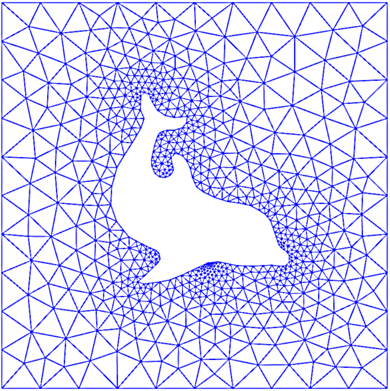
The idea of the finite element method is to divide the domain into triangles (elements) and seek a polynomial approximations to the unknown functions on each triangle. The method glues these piecewise approximations together to find a global solution. Linear and quadratic polynomials over the triangles are particularly popular, because of their mathematical simplicity, but higher-degree polynomials are advantageous to create very computationally efficient methods. The reason for using triangles is that they can easily approximate geometrically complicated domains, but quadrilateral elements and boxes in 3D are also widely used.