Approximation of functions in 2D

All the concepts and algorithms developed for approximation of 1D functions $ f(x) $ can readily be extended to 2D functions $ f(x,y) $ and 3D functions $ f(x,y,z) $. Basically, the extensions consist of defining basis functions $ \baspsi_i(x,y) $ or $ \baspsi_i(x,y,z) $ over some domain $ \Omega $, and for the least squares and Galerkin methods, the integration is done over $ \Omega $.

As in 1D, the least squares and projection/Galerkin methods lead to linear systems $$ \begin{align*} \sum_{j\in\If} A_{i,j}c_j &= b_i,\quad i\in\If,\\ A_{i,j} &= (\baspsi_i,\baspsi_j),\\ b_i &= (f,\baspsi_i), \end{align*} $$ where the inner product of two functions $ f(x,y) $ and $ g(x,y) $ is defined completely analogously to the 1D case (24): $$ \begin{equation} (f,g) = \int_\Omega f(x,y)g(x,y) dx dy \tag{114} \end{equation} $$

2D basis functions as tensor products of 1D functions

One straightforward way to construct a basis in 2D is to combine 1D basis functions. Say we have the 1D vector space $$ \begin{equation} V_x = \mbox{span}\{ \hat\baspsi_0(x),\ldots,\hat\baspsi_{N_x}(x)\} \tag{115} \tp \end{equation} $$ A similar space for a function's variation in $ y $ can be defined, $$ \begin{equation} V_y = \mbox{span}\{ \hat\baspsi_0(y),\ldots,\hat\baspsi_{N_y}(y)\} \tag{116} \tp \end{equation} $$ We can then form 2D basis functions as tensor products of 1D basis functions.

Tensor products. Given two vectors $ a=(a_0,\ldots,a_M) $ and $ b=(b_0,\ldots,b_N) $, their outer tensor product, also called the dyadic product, is $ p=a\otimes b $, defined through $$ p_{i,j}=a_ib_j,\quad i=0,\ldots,M,\ j=0,\ldots,N\tp$$ In the tensor terminology, $ a $ and $ b $ are first-order tensors (vectors with one index, also termed rank-1 tensors), and then their outer tensor product is a second-order tensor (matrix with two indices, also termed rank-2 tensor). The corresponding inner tensor product is the well-known scalar or dot product of two vectors: $ p=a\cdot b = \sum_{j=0}^N a_jb_j $. Now, $ p $ is a rank-0 tensor.

Tensors are typically represented by arrays in computer code. In the above example, $ a $ and $ b $ are represented by one-dimensional arrays of length $ M $ and $ N $, respectively, while $ p=a\otimes b $ must be represented by a two-dimensional array of size $ M\times N $.

Tensor products can be used in a variety of context.

Given the vector spaces $ V_x $ and $ V_y $ as defined in (115) and (116), the tensor product space $ V=V_x\otimes V_y $ has a basis formed as the tensor product of the basis for $ V_x $ and $ V_y $. That is, if $ \left\{ \basphi_i(x) \right\}_{i\in\Ix} $ and $ \left\{ \basphi_i(y) \right\}_{i\in \Iy} $ are basis for $ V_x $ and $ V_y $, respectively, the elements in the basis for $ V $ arise from the tensor product: $ \left\{ \basphi_i(x)\basphi_j(y) \right\}_{i\in \Ix,j\in \Iy} $. The index sets are $ I_x=\{0,\ldots,N_x\} $ and $ I_y=\{0,\ldots,N_y\} $.

The notation for a basis function in 2D can employ a double index as in $$ \baspsi_{p,q}(x,y) = \hat\baspsi_p(x)\hat\baspsi_q(y), \quad p\in\Ix,q\in\Iy\tp $$ The expansion for $ u $ is then written as a double sum $$ u = \sum_{p\in\Ix}\sum_{q\in\Iy} c_{p,q}\baspsi_{p,q}(x,y)\tp $$ Alternatively, we may employ a single index, $$ \baspsi_i(x,y) = \hat\baspsi_p(x)\hat\baspsi_q(y), $$ and use the standard form for $ u $, $$ u = \sum_{j\in\If} c_j\baspsi_j(x,y)\tp$$ The single index is related to the double index through $ i=p (N_y+1) + q $ or $ i=q (N_x+1) + p $.

Example: Polynomial basis in 2D

Suppose we choose $ \hat\baspsi_p(x)=x^p $, and try an approximation with $ N_x=N_y=1 $: $$ \baspsi_{0,0}=1,\quad \baspsi_{1,0}=x, \quad \baspsi_{0,1}=y, \quad \baspsi_{1,1}=xy \tp $$ Using a mapping to one index like $ i=q (N_x+1) + p $, we get $$ \baspsi_0=1,\quad \baspsi_1=x, \quad \baspsi_2=y,\quad\baspsi_3 =xy \tp $$

With the specific choice $ f(x,y) = (1+x^2)(1+2y^2) $ on $ \Omega = [0,L_x]\times [0,L_y] $, we can perform actual calculations: $$ \begin{align*} A_{0,0} &= (\baspsi_0,\baspsi_0) = \int_0^{L_y}\int_{0}^{L_x} \baspsi_0(x,y)^2 dx dy = \int_0^{L_y}\int_{0}^{L_x}dx dy = L_xL_y,\\ A_{1,0} &= (\baspsi_1,\baspsi_0) = \int_0^{L_y}\int_{0}^{L_x} x dxdy = {\half}L_x^2L_y,\\ A_{0,1} &= (\baspsi_0,\baspsi_1) = \int_0^{L_y}\int_{0}^{L_x} y dxdy = {\half}L_y^2L_x,\\ A_{0,1} &= (\baspsi_0,\baspsi_1) = \int_0^{L_y}\int_{0}^{L_x} xy dxdy = \int_0^{L_y}ydy \int_{0}^{L_x} xdx = \frac{1}{4}L_y^2L_x^2 \tp \end{align*} $$ The right-hand side vector has the entries $$ \begin{align*} b_{0} &= (\baspsi_0,f) = \int_0^{L_y}\int_{0}^{L_x}1\cdot (1+x^2)(1+2y^2) dxdy\\ &= \int_0^{L_y}(1+2y^2)dy \int_{0}^{L_x} (1+x^2)dx = (L_y + \frac{2}{3}L_y^3)(L_x + \frac{1}{3}L_x^3)\\ b_{1} &= (\baspsi_1,f) = \int_0^{L_y}\int_{0}^{L_x} x(1+x^2)(1+2y^2) dxdy\\ &=\int_0^{L_y}(1+2y^2)dy \int_{0}^{L_x} x(1+x^2)dx = (L_y + \frac{2}{3}L_y^3)({\half}L_x^2 + \frac{1}{4}L_x^4)\\ b_{2} &= (\baspsi_2,f) = \int_0^{L_y}\int_{0}^{L_x} y(1+x^2)(1+2y^2) dxdy\\ &= \int_0^{L_y}y(1+2y^2)dy \int_{0}^{L_x} (1+x^2)dx = ({\half}L_y + {\half}L_y^4)(L_x + \frac{1}{3}L_x^3)\\ b_{3} &= (\baspsi_2,f) = \int_0^{L_y}\int_{0}^{L_x} xy(1+x^2)(1+2y^2) dxdy\\ &= \int_0^{L_y}y(1+2y^2)dy \int_{0}^{L_x} x(1+x^2)dx = ({\half}L_y^2 + {\half}L_y^4)({\half}L_x^2 + \frac{1}{4}L_x^4) \tp \end{align*} $$

There is a general pattern in these calculations that we can explore. An arbitrary matrix entry has the formula $$ \begin{align*} A_{i,j} &= (\baspsi_i,\baspsi_j) = \int_0^{L_y}\int_{0}^{L_x} \baspsi_i\baspsi_j dx dy \\ &= \int_0^{L_y}\int_{0}^{L_x} \baspsi_{p,q}\baspsi_{r,s} dx dy = \int_0^{L_y}\int_{0}^{L_x} \hat\baspsi_p(x)\hat\baspsi_q(y)\hat\baspsi_r(x)\hat\baspsi_s(y) dx dy\\ &= \int_0^{L_y} \hat\baspsi_q(y)\hat\baspsi_s(y)dy \int_{0}^{L_x} \hat\baspsi_p(x) \hat\baspsi_r(x) dx\\ &= \hat A^{(x)}_{p,r}\hat A^{(y)}_{q,s}, \end{align*} $$ where $$ \hat A^{(x)}_{p,r} = \int_{0}^{L_x} \hat\baspsi_p(x) \hat\baspsi_r(x) dx, \quad \hat A^{(y)}_{q,s} = \int_0^{L_y} \hat\baspsi_q(y)\hat\baspsi_s(y)dy, $$ are matrix entries for one-dimensional approximations. Moreover, $ i=q N_y+q $ and $ j=s N_y+r $.

With $ \hat\baspsi_p(x)=x^p $ we have $$ \hat A^{(x)}_{p,r} = \frac{1}{p+r+1}L_x^{p+r+1},\quad \hat A^{(y)}_{q,s} = \frac{1}{q+s+1}L_y^{q+s+1}, $$ and $$ A_{i,j} = \hat A^{(x)}_{p,r} \hat A^{(y)}_{q,s} = \frac{1}{p+r+1}L_x^{p+r+1} \frac{1}{q+s+1}L_y^{q+s+1}, $$ for $ p,r\in\Ix $ and $ q,s\in\Iy $.

Corresponding reasoning for the right-hand side leads to $$ \begin{align*} b_i &= (\baspsi_i,f) = \int_0^{L_y}\int_{0}^{L_x}\baspsi_i f\,dxdx\\ &= \int_0^{L_y}\int_{0}^{L_x}\hat\baspsi_p(x)\hat\baspsi_q(y) f\,dxdx\\ &= \int_0^{L_y}\hat\baspsi_q(y) (1+2y^2)dy \int_0^{L_y}\hat\baspsi_p(x) x^p (1+x^2)dx\\ &= \int_0^{L_y} y^q (1+2y^2)dy \int_0^{L_y}x^p (1+x^2)dx\\ &= (\frac{1}{q+1} L_y^{q+1} + \frac{2}{q+3}L_y^{q+3}) (\frac{1}{p+1} L_x^{p+1} + \frac{2}{q+3}L_x^{p+3}) \end{align*} $$

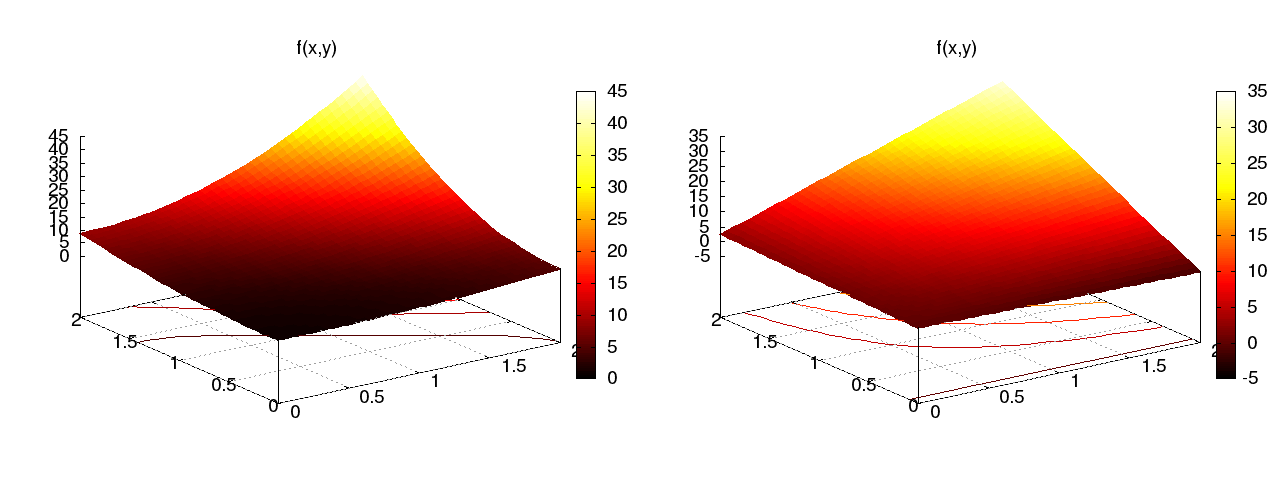
Choosing $ L_x=L_y=2 $, we have $$ A = \left[\begin{array}{cccc} 4 & 4 & 4 & 4\\ 4 & \frac{16}{3} & 4 & \frac{16}{3}\\ 4 & 4 & \frac{16}{3} & \frac{16}{3}\\ 4 & \frac{16}{3} & \frac{16}{3} & \frac{64}{9} \end{array}\right],\quad b = \left[\begin{array}{c} \frac{308}{9}\\\frac{140}{3}\\44\\60\end{array}\right], \quad c = \left[ \begin{array}{r} -\frac{1}{9} \\ \frac{4}{3} \\ - \frac{2}{3} \\ 8 \end{array}\right] \tp $$ Figure 35 illustrates the result.

Figure 35: Approximation of a 2D quadratic function (left) by a 2D bilinear function (right) using the Galerkin or least squares method.

Implementation

The least_squares function from the section Orthogonal basis functions and/or the file approx1D.py can with very small modifications solve 2D approximation problems. First, let Omega now be a list of the intervals in $ x $ and $ y $ direction. For example, $ \Omega = [0,L_x]\times [0,L_y] $ can be represented by Omega = [[0, L_x], [0, L_y]].

Second, the symbolic integration must be extended to 2D:

import sympy as sym

integrand = psi[i]*psi[j]
I = sym.integrate(integrand,
                 (x, Omega[0][0], Omega[0][1]),
                 (y, Omega[1][0], Omega[1][1]))

provided integrand is an expression involving the sympy symbols x and y. The 2D version of numerical integration becomes

if isinstance(I, sym.Integral):
    integrand = sym.lambdify([x,y], integrand)
    I = sym.mpmath.quad(integrand,
                       [Omega[0][0], Omega[0][1]],
                       [Omega[1][0], Omega[1][1]])

The right-hand side integrals are modified in a similar way. (We should add that sympy.mpmath.quad is sufficiently fast even in 2D, but scipy.integrate.nquad is much faster.)

Third, we must construct a list of 2D basis functions. Here are two examples based on tensor products of 1D "Taylor-style" polynomials $ x^i $ and 1D sine functions $ \sin((i+1)\pi x) $:

def taylor(x, y, Nx, Ny):
    return [x**i*y**j for i in range(Nx+1) for j in range(Ny+1)]

def sines(x, y, Nx, Ny):
    return [sym.sin(sym.pi*(i+1)*x)*sym.sin(sym.pi*(j+1)*y)
            for i in range(Nx+1) for j in range(Ny+1)]

The complete code appears in approx2D.py.

The previous hand calculation where a quadratic $ f $ was approximated by a bilinear function can be computed symbolically by

>>> from approx2D import *
>>> f = (1+x**2)*(1+2*y**2)
>>> psi = taylor(x, y, 1, 1)
>>> Omega = [[0, 2], [0, 2]]
>>> u, c = least_squares(f, psi, Omega)
>>> print u
8*x*y - 2*x/3 + 4*y/3 - 1/9
>>> print sym.expand(f)
2*x**2*y**2 + x**2 + 2*y**2 + 1

We may continue with adding higher powers to the basis:

>>> psi = taylor(x, y, 2, 2)
>>> u, c = least_squares(f, psi, Omega)
>>> print u
2*x**2*y**2 + x**2 + 2*y**2 + 1
>>> print u-f
0

For $ N_x\geq 2 $ and $ N_y\geq 2 $ we recover the exact function $ f $, as expected, since in that case $ f\in V $ (see the section Perfect approximation).

Extension to 3D

Extension to 3D is in principle straightforward once the 2D extension is understood. The only major difference is that we need the repeated outer tensor product, $$ V = V_x\otimes V_y\otimes V_z\tp$$ In general, given vectors (first-order tensors) $ a^{(q)} = (a^{(q)}_0,\ldots,a^{(q)}_{N_q} $, $ q=0,\ldots,m $, the tensor product $ p=a^{(0)}\otimes\cdots\otimes a^{m} $ has elements $$ p_{i_0,i_1,\ldots,i_m} = a^{(0)}_{i_1}a^{(1)}_{i_1}\cdots a^{(m)}_{i_m}\tp$$ The basis functions in 3D are then $$ \baspsi_{p,q,r}(x,y,z) = \hat\baspsi_p(x)\hat\baspsi_q(y)\hat\baspsi_r(z),$$ with $ p\in\Ix $, $ q\in\Iy $, $ r\in\Iz $. The expansion of $ u $ becomes $$ u(x,y,z) = \sum_{p\in\Ix}\sum_{q\in\Iy}\sum_{r\in\Iz} c_{p,q,r} \baspsi_{p,q,r}(x,y,z)\tp$$ A single index can be introduced also here, e.g., $ i=N_xN_yr + q_Nx + p $, $ u=\sum_i c_i\baspsi_i(x,y,z) $.

Use of tensor product spaces. Constructing a multi-dimensional space and basis from tensor products of 1D spaces is a standard technique when working with global basis functions. In the world of finite elements, constructing basis functions by tensor products is much used on quadrilateral and hexahedra cell shapes, but not on triangles and tetrahedra. Also, the global finite element basis functions are almost exclusively denoted by a single index and not by the natural tuple of indices that arises from tensor products.