A generalized element concept
So far, finite element computing has employed the nodes and
element lists together with the definition of the basis functions
in the reference element. Suppose we want to introduce a piecewise
constant approximation with one basis function \( \refphi_0(x)=1 \) in
the reference element, corresponding to a \( \basphi_i(x) \) function that
is 1 on element number \( i \) and zero on all other elements.
Although we could associate the function value
with a node in the middle of the elements, there are no nodes at the
ends, and the previous code snippets will not work because we
cannot find the element boundaries from the nodes list.
In order to get a richer space of finite element approximations, we need to revise the simple node and element concept presented so far and introduce a more powerful terminology. Much literature employs the definition of node and element introduced in the previous sections so it is important have this knowledge, besides being a good pedagogical background from understanding the extended element concept in the following.
Cells, vertices, and degrees of freedom
We now introduce cells as the subdomains \( \Omega^{(e)} \) previously referred to as elements. The cell boundaries are denoted as vertices. The reason for this name is that cells are recognized by their vertices in 2D and 3D. We also define a set of degrees of freedom (dof), which are the quantities we aim to compute. The most common type of degree of freedom is the value of the unknown function \( u \) at some point. (For example, we can introduce nodes as before and say the degrees of freedom are the values of \( u \) at the nodes.) The basis functions are constructed so that they equal unity for one particular degree of freedom and zero for the rest. This property ensures that when we evaluate \( u=\sum_j c_j\basphi_j \) for degree of freedom number \( i \), we get \( u=c_i \). Integrals are performed over cells, usually by mapping the cell of interest to a reference cell.
With the concepts of cells, vertices, and degrees of freedom we increase the decoupling of the geometry (cell, vertices) from the space of basis functions. We will associate different sets of basis functions with a cell. In 1D, all cells are intervals, while in 2D we can have cells that are triangles with straight sides, or any polygon, or in fact any two-dimensional geometry. Triangles and quadrilaterals are most common, though. The popular cell types in 3D are tetrahedra and hexahedra.
Extended finite element concept
The concept of a finite element is now
- a reference cell in a local reference coordinate system;
- a set of basis functions \( \refphi_i \) defined on the cell;
- a set of degrees of freedom that uniquely determines the basis functions such that \( \refphi_i=1 \) for degree of freedom number \( i \) and \( \refphi_i=0 \) for all other degrees of freedom;
- a mapping between local and global degree of freedom numbers, here called the dof map;
- a geometric mapping of the reference cell onto the cell in the physical domain.
The expansion of \( u \) over one cell is often used: $$ \begin{equation} u(x) = \tilde u(X) = \sum_{r} c_r\refphi_r(X),\quad x\in\Omega^{(e)},\ X\in [-1,1], \tag{100} \end{equation} $$ where the sum is taken over the numbers of the degrees of freedom and \( c_r \) is the value of \( u \) for degree of freedom number \( r \).
Our previous P1, P2, etc., elements are defined by introducing \( d+1 \)
equally spaced nodes in the reference cell and saying that the degrees
of freedom are the \( d+1 \) function values at these nodes. The basis
functions must be 1 at one node and 0 at the others, and the Lagrange
polynomials have exactly this property. The nodes can be numbered
from left to right with associated degrees of freedom that are
numbered in the same way. The degree of freedom mapping becomes what
was previously represented by the elements lists. The cell mapping
is the same affine mapping (70) as
before.
Implementation
Implementationwise,
- we replace
nodesbyvertices; - we introduce
cellssuch thatcell[e][r]gives the mapping from local vertexrin celleto the global vertex number invertices; - we replace
elementsbydof_map(the contents are the same for Pd elements).
vertices = [0, 0.4, 1]
cells = [[0, 1], [1, 2]]
dof_map = [[0, 1, 2], [2, 3, 4]]
If we would approximate \( f \) by piecewise constants, known as
P0 elements, we simply
introduce one point or node in an element, preferably \( X=0 \),
and define one degree of freedom, which is the function value
at this node. Moreover, we set \( \refphi_0(X)=1 \).
The cells and vertices arrays remain the same, but
dof_map is altered:
dof_map = [[0], [1]]
We use the cells and vertices lists to retrieve information
on the geometry of a cell, while dof_map is the
\( q(e,r) \) mapping introduced earlier in the
assembly of element matrices and vectors.
For example, the Omega_e variable (representing the cell interval)
in previous code snippets must now be computed as
Omega_e = [vertices[cells[e][0], vertices[cells[e][1]]
The assembly is done by
A[dof_map[e][r], dof_map[e][s]] += A_e[r,s]
b[dof_map[e][r]] += b_e[r]
We will hereafter drop the nodes and elements arrays
and work exclusively with cells, vertices, and dof_map.
The module fe_approx1D_numint.py now replaces the module
fe_approx1D and offers similar functions that work with
the new concepts:
from fe_approx1D_numint import *
x = sym.Symbol('x')
f = x*(1 - x)
N_e = 10
vertices, cells, dof_map = mesh_uniform(N_e, d=3, Omega=[0,1])
phi = [basis(len(dof_map[e])-1) for e in range(N_e)]
A, b = assemble(vertices, cells, dof_map, phi, f)
c = np.linalg.solve(A, b)
# Make very fine mesh and sample u(x) on this mesh for plotting
x_u, u = u_glob(c, vertices, cells, dof_map,
                resolution_per_element=51)
plot(x_u, u)
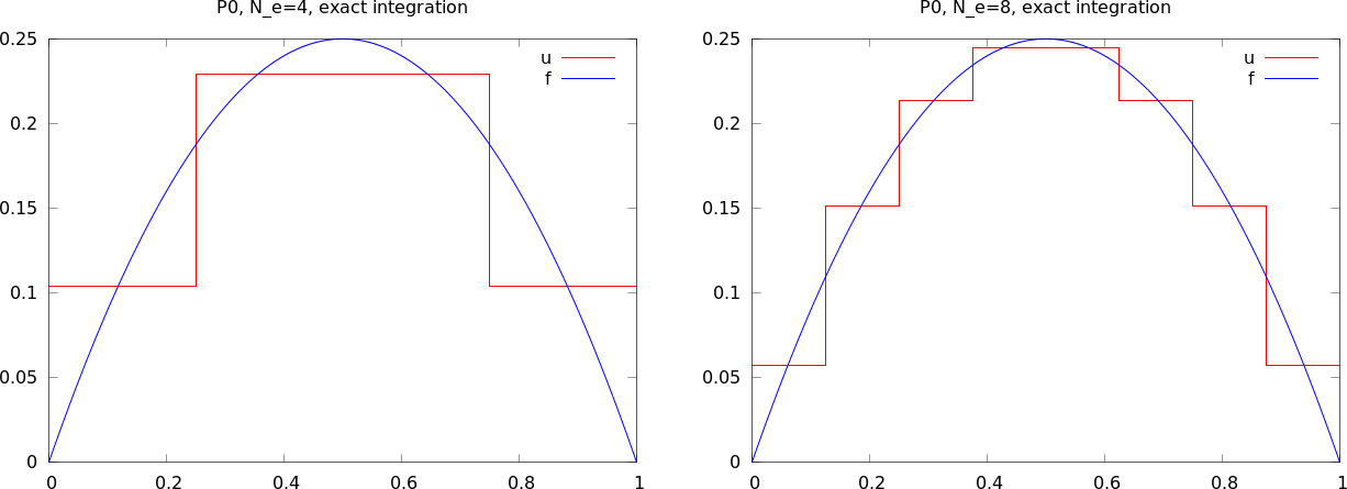
These steps are offered in the approximate function, which we here
apply to see how well four P0 elements (piecewise constants)
can approximate a parabola:
from fe_approx1D_numint import *
x=sym.Symbol("x")
for N_e in 4, 8:
    approximate(x*(1-x), d=0, N_e=N_e, Omega=[0,1])
Figure 34 shows the result.
Figure 34: Approximation of a parabola by 4 (left) and 8 (right) P0 elements.
Computing the error of the approximation
So far we have focused on computing the coefficients \( c_j \) in the
approximation \( u(x)=\sum_jc_j\basphi_j \) as well as on plotting \( u \) and
\( f \) for visual comparison. A more quantitative comparison needs to
investigate the error \( e(x)=f(x)-u(x) \). We mostly want a single number to
reflect the error and use a norm for this purpose, usually the \( L^2 \) norm
$$ ||e||_{L^2} = \left(\int_{\Omega} e^2 \dx\right)^{1/2}\tp$$
Since the finite element approximation is defined for all \( x\in\Omega \),
and we are interested in how \( u(x) \) deviates from \( f(x) \) through all
the elements,
we can either integrate analytically or use an accurate numerical
approximation. The latter is more convenient as it is a generally
feasible and simple approach. The idea is to sample \( e(x) \)
at a large number of points in each element. The function u_glob
in the fe_approx1D_numint module does this for \( u(x) \) and returns
an array x with coordinates and an array u with the \( u \) values:
x, u = u_glob(c, vertices, cells, dof_map,
              resolution_per_element=101)
e = f(x) - u
Let us use the Trapezoidal method to approximate the integral. Because
different elements may have different lengths, the x array has
a non-uniformly distributed set of coordinates. Also, the u_glob
function works in an element by element fashion such that coordinates
at the boundaries between elements appear twice. We therefore need
to use a "raw" version of the Trapezoidal rule where we just add up
all the trapezoids:
$$ \int_\Omega g(x) \dx \approx \sum_{j=0}^{n-1} \half(g(x_j) +
g(x_{j+1}))(x_{j+1}-x_j),$$
if \( x_0,\ldots,x_n \) are all the coordinates in x. In
vectorized Python code,
g_x = g(x)
integral = 0.5*np.sum((g_x[:-1] + g_x[1:])*(x[1:] - x[:-1]))
Computing the \( L^2 \) norm of the error, here named E, is now achieved by
e2 = e**2
E = np.sqrt(0.5*np.sum((e2[:-1] + e2[1:])*(x[1:] - x[:-1]))
Example: Cubic Hermite polynomials
The finite elements considered so far represent \( u \) as piecewise polynomials with discontinuous derivatives at the cell boundaries. Sometimes it is desirable to have continuous derivatives. A primary example is the solution of differential equations with fourth-order derivatives where standard finite element formulations lead to a need for basis functions with continuous first-order derivatives. The most common type of such basis functions in 1D is the so-called cubic Hermite polynomials. The construction of such polynomials, as explained next, will further exemplify the concepts of a cell, vertex, degree of freedom, and dof map.
Given a reference cell \( [-1,1] \), we seek cubic polynomials with the values of the function and its first-order derivative at \( X=-1 \) and \( X=1 \) as the four degrees of freedom. Let us number the degrees of freedom as
- 0: value of function at \( X=-1 \)
- 1: value of first derivative at \( X=-1 \)
- 2: value of function at \( X=1 \)
- 3: value of first derivative at \( X=1 \)
The four basis functions can be written in a general form $$ \refphi_i (X) = \sum_{j=0}^3 C_{i,j}X^j, $$ with four coefficients \( C_{i,j} \), \( j=0,1,2,3 \), to be determined for each \( i \). The constraints that basis function number \( i \) must be 1 for degree of freedom number \( i \) and zero for the other three degrees of freedom, gives four equations to determine \( C_{i,j} \) for each \( i \). In mathematical detail, $$ \begin{align*} \refphi_0 (-1) &= 1,\quad \refphi_0 (1)=\refphi_0'(-1)=\refphi_i' (1)=0,\\ \refphi_1' (-1) &= 1,\quad \refphi_1 (-1)=\refphi_1(1)=\refphi_1' (1)=0,\\ \refphi_2 (1) &= 1,\quad \refphi_2 (-1)=\refphi_2'(-1)=\refphi_2' (1)=0,\\ \refphi_3' (1) &= 1,\quad \refphi_3 (-1)=\refphi_3'(-1)=\refphi_3 (1)=0 \tp \end{align*} $$ These four \( 4\times 4 \) linear equations can be solved, yielding the following formulas for the cubic basis functions: $$ \begin{align} \refphi_0(X) &= 1 - \frac{3}{4}(X+1)^2 + \frac{1}{4}(X+1)^3 \tag{102}\\ \refphi_1(X) &= -(X+1)(1 - \half(X+1))^2 \tag{103}\\ \refphi_2(X) &= \frac{3}{4}(X+1)^2 - \half(X+1)^3 \tag{104}\\ \refphi_3(X) &= -\half(X+1)(\half(X+1)^2 - (X+1)) \tag{105}\\ \tag{106} \end{align} $$
The construction of the dof map needs a scheme for numbering the global degrees of freedom. A natural left-to-right numbering has the function value at vertex \( \xno{i} \) as degree of freedom number \( 2i \) and the value of the derivative at \( \xno{i} \) as degree of freedom number \( 2i+1 \), \( i=0,\ldots,N_e+1 \).