Visual exploration
This section explains how to load the data from the computation, stored
as a pickled list in the file bumpy.res, into various arrays, and how
to visualize these arrays. We want to produce the following plots:
- \( u(t) \) and \( u'(t) \) for \( t\geq t_s \)
- the spectrum of \( u(t) \), for \( t\geq t_s \) (using FFT) to see which frequencies that dominate in the signal
- for each road shape, a plot of \( h(x) \), \( a(t) \), and \( u(t) \), for \( t \geq t_s \)
Test case
The simulation is run as
Terminal> python bumpy.py --v 10
meaning that all other parameters have their default values as
specified in the command_line_arguments function.
Importing array and plot functionality
The following two imports give access to Matlab-style functions for plotting and computing with arrays:
from numpy import *
from matplotlib.pyplot import *
The Python community often prefers to prefix numpy by np and
matplotlib by plt or mpl:
import numpy as np
import matplotlib.pyplot as plt
However, we shall stick to the former import to make the code as close as possible to the Matlab equivalent.
Reading results from file
Loading the computational data from file back to a list data must
use the same module (cPickle or dill) as we used for writing the data:
import cPickle as pickle
# or
import dill as pickle
outfile = open('bumpy.res', 'r')
data = pickle.load(outfile)
outfile.close()

x, t = data[0:2]
Note that data first contains x and t, thereafter
a sequence of 3-lists [h, F, u]. With data[0:2] we extract
the sublist with elements data[0] and data[1] (0:2 means
up to, but not including 2).
All the remaining 3-lists [h, F, u] can be extracted as data[2:].
Since now we concentrate on the part \( t\geq t_s \) of the data, we can grab the corresponding parts of the arrays in the following way, using boolean arrays as indices:
indices = t >= t_s   # True/False boolean array
t = t[indices]       # fetch the part of t for which t >= t_s
x = x[indices]       # fetch the part of x for which t >= t_s
Indexing by a boolean array extracts all the elements corresponding to
the True elements in the index array.
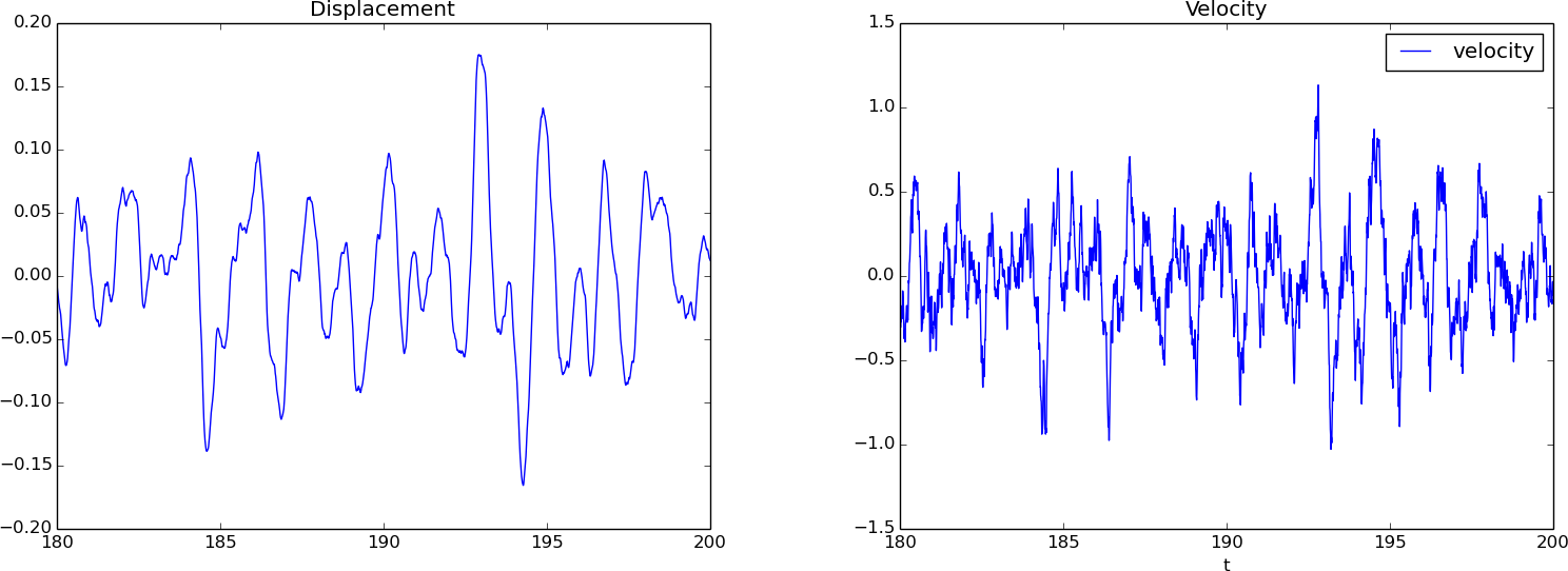
Plotting \( u \)
A plot of \( u \), corresponding to the second realization of the bumpy road, is easy to create:
figure()
realization = 1
u = data[2+realization][2][indices]
plot(t, u)
title('Displacement')
Note that data[2:] holds the triplets [h,F,u], so the second
realization is data[3]. The u part of the triplet is then data[3][2],
and the part of u where \( t\geq t_s \) is then data[3][2][indices].
Figure 3 (left) shows the result.
Computing and plotting \( u' \)
Given a discrete function \( u^n \), \( n=0,\ldots,N \), the corresponding discrete derivative can be computed by $$ \begin{equation} v^n = \frac{u^{n+1}-u^{n-1}}{2\Delta t},\quad n=1,\ldots,N-1\thinspace . \tag{6} \end{equation} $$ The values at the end points, \( v^0 \) and \( v^N \), must be computed with less accurate one-sided differences: $$ v^0 = \frac{u^1-u^0}{\Delta t},\quad v^{N} = \frac{u^N-u^{N-1}}{\Delta t}$$
Computing \( v=u' \) by (6) for the part \( t\geq t_s \) is done by
v = zeros_like(u)           # same length and data type as u
dt = t[1] - t[0]            # time step
for i in range(1,u.size-1):
    v[i] = (u[i+1] - u[i-1])/(2*dt)
v[0] = (u[1] - u[0])/dt
v[N] = (u[N] - u[N-1])/dt
Plotting of v is done by
figure()
plot(t, v)
legend(['velocity'])
xlabel('t')
title('Velocity')
Figure 3 (right) shows that the velocity is much more "noisy" than the displacement.
Figure 3: Displacement (left) and velocity (right) for \( t\geq t_s=180 \).
Vectorized computation of \( u' \)
For large arrays, finite difference formulas like (6) can be heavy to compute. A vectorized expression where the loop is avoided is much more efficient:
v = zeros_like(u)
v[1:-1] = (u[2:] - u[:-2])/(2*dt)
v[0] = (u[1] - u[0])/dt
v[-1] = (u[-1] - u[-2])/dt
The challenging expression here is u[2:] - u[:-2].
The array slice u[2:] starts at index 2 and goes to the very end of
the array, i.e., the slice contains u[2], u[3], ..., u[N].
The slice u[:-2] starts from the beginning of u and goes up to,
but not including the second last element, i.e.,
u[0], u[1], ..., u[N-2]. The expression u[2:] - u[:-2] is then
an array of length N-2 with elements
u[2]-u[0], u[3]-u[1], and so on, and with u[N]-u[N-2] as final
element. After dividing this array by 2*dt we have evaluated formula
(6) for all indices from 1 to N-2, which
is the same as the slice 1:-1 (used on the left-hand side).
Rather than using N (equal to u.size-1) in the last line above,
we use the -1 index for the last element and -2 for the second
last element.
How efficient is this vectorization? The interactive IPython shell has a convenient feature to test the efficiency of Python constructions:
In [1]: from numpy import zeros

In [2]: N = 1000000

In [3]: u = zeros(N)

In [4]: %timeit v = u[2:] - u[:-2]
1 loops, best of 3: 5.76 ms per loop

In [5]: v = zeros(N)

In [6]: %timeit for i in range(1,N-1): v[i] = u[i+1] - u[i-1]
1 loops, best of 3: 836 ms per loop

In [7]: 836/5.76
Out[20]: 145.13888888888889
This session show that the vectorized expression is 145 times faster than the explicit loop!
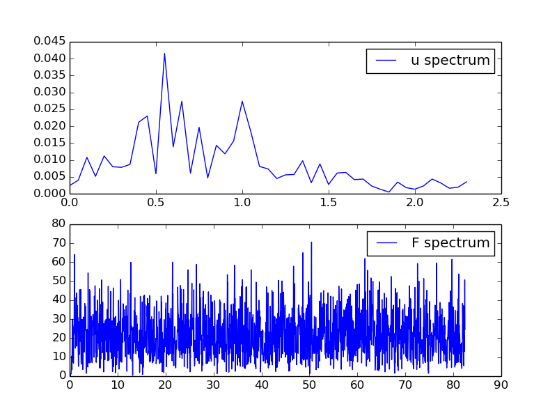
Computing the spectrum of signals
The spectrum of a \( u(t) \) function, here represented by discrete values in
the arrays u and t, can be computed by the Python function
def frequency_analysis(u, t):
    A = fft(u)
    A = 2*A
    dt = t[1] - t[0]
    N = t.size
    freq = arange(N/2, dtype=float)/N/dt
    A = abs(A[0:freq.size])/N
    # Remove small high frequency part
    tol = 0.05*A.max()
    for i in xrange(len(A)-1, 0, -1):
        if A[i] > tol:
            break
    return freq[:i+1], A[:i+1]
Note here that we truncate that last part of the spectrum where the amplitudes are small (this usually gives a plot that is easier to inspect).
In the present case, we utilize the frequency_analysis through
figure()
u = data[3][2][indices]  # second realization of u
f, A = frequency_analysis(u, t)
plot(f, A)
title('Spectrum of u')
Figure 4 shows the amplitudes and that the dominating frequencies lie around 0.5 and 1 Hz.
Figure 4: Spectra of displacement and excitation.
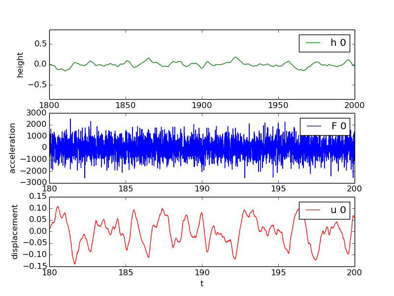
Multiple plots in the same figure
Finally, we can run through all the 3-lists [h, a, u] and visualize
these curves in the same plot figure:
for realization in range(len(data[2:])):
    h, F, u = data[2+realization]
    h = h[indices]
    F = F[indices]
    u = u[indices]

    figure()
    subplot(3, 1, 1)
    plot(x, h, 'g-')
    legend(['h %d' % realization])
    hmax = (abs(h.max()) + abs(h.min()))/2
    axis([x[0], x[-1], -hmax*5, hmax*5])
    xlabel('distance'); ylabel('height')

    subplot(3, 1, 2)
    plot(t, F)
    legend(['F %d' % realization])
    xlabel('t'); ylabel('acceleration')

    subplot(3, 1, 3)
    plot(t, u, 'r-')
    legend(['u %d' % realization])
    xlabel('t'); ylabel('displacement')
    savefig('hFu%d.png' % realization)
Figure 5: First realization of a bumpy road, with corresponding excitation of the wheel and resulting vertical vibrations.
If all the plot commands above are placed in a file, as in
explore.py, a final show() call is needed to show the
plots on the screen. On the other hand, the commands are usually
more conveniently performed in an interactive Python shell, preferably
IPython or IPython notebook.