Simple implementation

Let us first implement the computational formulas for the linear damping case in a short and compact Python function:

from numpy import *

def solver_linear_damping(I, V, m, b, s, F, t):
    N = t.size - 1              # No of time intervals
    dt = t[1] - t[0]            # Time step
    u = zeros(N+1)              # Result array
    u[0] = I
    u[1] = u[0] + dt*V + dt**2/(2*m)*(-b*V - s(u[0]) + F[0])

    for n in range(1,N):
        u[n+1] = 1./(m + b*dt/2)*(2*m*u[n] + \ 
                 (b*dt/2 - m)*u[n-1] + dt**2*(F[n] - s(u[n])))
    return u

Dissection of the code

Functions in Python start with def, followed by the function name and the list of input objects separated by comma. The function body is indented, and the first non-indented line signifies the end of the function body block. Output objects are returned to the calling code by a return statement.

The arguments to this function and the variables created inside the function are not declared with type. We therefore need to know what the variables are supposed to be: I, V, m, and b are real numbers, while F and t are one-dimensional arrays of the same length, where F holds \( F(t_n) \) and t holds \( t_n \), \( n=0,1,\ldots,N+1 \).

The number of elements in an array t is given by t.size (or len(t), but t.size works for multi-dimensional arrays too). Arrays are indexed by square brackets, and indices always start at 0. Numerical codes frequently needs to loop over array indices, i.e., a set of integers. Such a set is produced by range(start, stop, increment), which returns a list of integers start, start+increment, start+2*increment, and so on, up to but not including stop. Writing just range(stop) means range(0, stop, 1). The particular call range(1, N) used in the code above results in a list of integers: 1, 2, ..., N-1.

Array functionality is enabled by the numpy package, which offers functions such as zeros and linspace, as known from Matlab. Here we import all objects in the numpy package by the statement

from numpy import *

Comments start with the character # and the rest of the line is then ignored by Python.

Every variable in Python is an object. In particular, the s function above is a function object, transferred to the function as any other object, and called as any other function. Transferring a function as argument to another function is therefore simpler and cleaner in Python than in, e.g., C, C++, Java, C#, and Matlab.

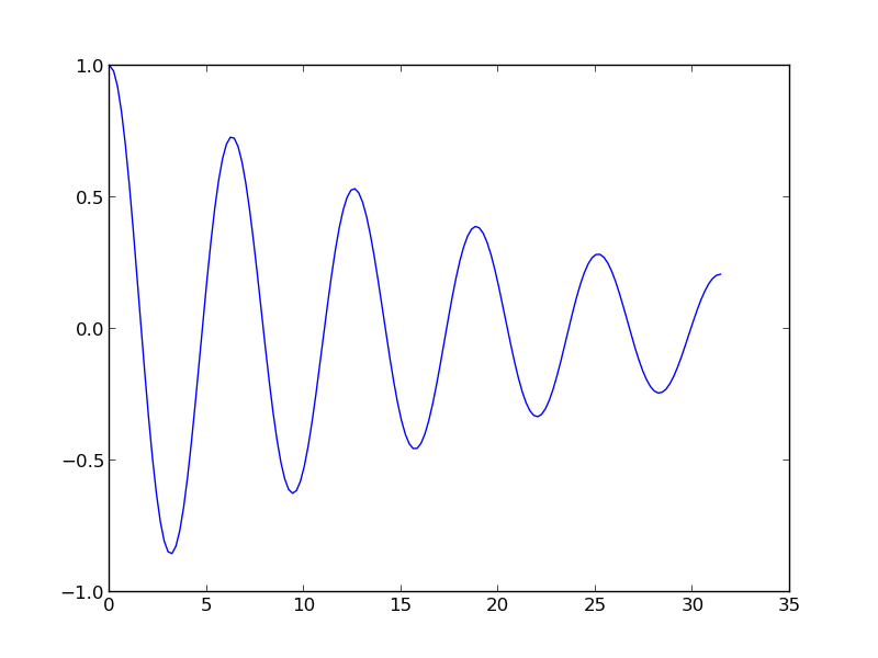
How can we use the solver_linear_damping function? We need to call it with relevant values for the arguments. Suppose we want to solve a vibration problem with \( I=1 \), \( V=0 \), \( F=0 \), \( m=2 \), \( b=0.2 \), \( s(u)=2u \), \( \Delta t=0.2 \), for \( t\in [0,10\pi] \). This will be a damped sinusoidal solution (setting \( b=0 \) will result in \( u(t)=\cos t \)). The test code becomes

from solver import solver_linear_damping
from numpy import *

def s(u):
    return 2*u

T = 10*pi      # simulate for t in [0,T]
dt = 0.2
N = int(round(T/dt))
t = linspace(0, T, N+1)
F = zeros(t.size)
I = 1; V = 0
m = 2; b = 0.2
u = solver_linear_damping(I, V, m, b, s, F, t)

from matplotlib.pyplot import *
plot(t, u)
savefig('tmp.pdf')   # save plot to PDF file
savefig('tmp.png')   # save plot to PNG file
show()

The solver_linear_damping function resides in the file solver.py, so if we make the call to this function in separate file (assumed above), we have to import the function as shown. We also need functions and variables from the numpy package, here pi, linspace, and zeros. Normally, there is one statement per line in Python programs, and there is no need to end the statement with a semicolon. However, if we want multiple statements on a line, they must be separated by semi colon as demonstrated in the initialization of I and V. Plotting the computed curve makes use of the matplotlib package, where we call its plot, savefig, and show functions. Figure 2 shows the result.

• «
• 1
• 2
• 3
• 4
• 5
• 6
• 7
• 8
• 9
• 10
• 11
• »