Operator splitting methods
Operator splitting is a natural and old idea. When a PDE or system of PDEs contains different terms expressing different physics, it is natural to use different numerical methods for different physical processes. This can optimize and simplify the overall solution process. The idea was especially popularized in the context of the Navier-Stokes equations and reaction-diffusion PDEs. Common names for the technique are operator splitting, fractional step methods, and split-step methods. We shall stick to the former name. In the context of nonlinear differential equations, operator splitting can be used to isolate nonlinear terms and simplify the solution methods.
A related technique, often known as dimensional splitting or alternating direction implicit (ADI) methods, is to split the spatial dimensions and solve a 2D or 3D problem as two or three consecutive 1D problems, but this type of splitting is not to be further considered here.
Ordinary operator splitting for ODEs
Consider first an ODE where the right-hand side is split into two terms: $$ \begin{equation} u' = f_0(u) + f_1(u)\tp \tag{5.71} \end{equation} $$ In case \( f_0 \) and \( f_1 \) are linear functions of \( u \), \( f_0=au \) and \( f_1=bu \), we have \( u(t)=Ie^{(a+b)t} \), if \( u(0)=I \). When going one time step of length \( \Delta t \) from \( t_n \) to \( t_{n+1} \), we have $$ u(t_{n+1}) = u(t_n)e^{(a+b)\Delta t}\tp$$ This expression can be also be written as $$ u(t_{n+1}) = u(t_n)e^{a\Delta t}e^{b\Delta t},$$ or $$ \begin{align} u^\stepzero &= u(t_n)e^{a\Delta t}, \tag{5.72}\\ u(t_{n+1}) &= u^\stepzero e^{b\Delta t} \tag{5.73} \end{align} $$ The first step (5.72) means solving \( u'=f_0 \) over a time interval \( \Delta t \) with \( u(t_n) \) as start value. The second step (5.73) means solving \( u'=f_1 \) over a time interval \( \Delta t \) with the value at the end of the first step as start value. That is, we progress the solution in two steps and solve two ODEs \( u'=f_0 \) and \( u'=f_1 \). The order of the equations is not important. From the derivation above we see that solving \( u'=f_1 \) prior to \( u'=f_0 \) can equally well be done.
The technique is exact if the ODEs are linear. For nonlinear ODEs it is only an approximate method with error \( \Delta t \). The technique can be extended to an arbitrary number of steps; i.e., we may split the PDE system into any number of subsystems. Examples will illuminate this principle.
Strang splitting for ODEs
The accuracy of the splitting method in the section Ordinary operator splitting for ODEs can be improved from \( \Oof{\Delta t} \) to \( \Oof{\Delta t^2} \) using so-called Strang splitting, where we take half a step with the \( f_0 \) operator, a full step with the \( f_1 \) operator, and finally half another step with the \( f_0 \) operator. During a time interval \( \Delta t \) the algorithm can be written as follows. $$ \begin{align*} \frac{du^{\stepzero}}{dt} &= f_0(u^{\stepzero}), \quad u^{\stepzero}(t_n)=u(t_n), \quad t\in [t_n,t_n+\half\Delta t],\\ \frac{du^{\stephalf}}{dt} &= f_1(u^{\stephalf}), \quad u^{\stephalf}(t_n)=u^{\stepzero}(t_{n+\half}), \quad t\in [t_n,t_n+\Delta t],\\ \frac{du^{\stepone}}{dt} &= f_0(u^{\stepone}), \quad u^{\stepone}(t_n+\half)=u^{\stephalf}(t_{n+\half}), \quad t\in [t_n+\half\Delta t, t_n+\Delta t]\tp \end{align*} $$ The global solution is set as \( u(t_{n+1}) = u^{\stepone}(t_{n+1}) \).
There is no use in combining higher-order methods with ordinary splitting since the error due to splitting is \( \Oof{\Delta t} \), but for Strang splitting it makes sense to use schemes of order \( \Oof{\Delta t^2} \).
With the notation introduced for Strang splitting, we may express ordinary first-order splitting as $$ \begin{align*} \frac{du^{\stepzero}}{dt} &= f_0(u^{\stepzero}),\quad u^{\stepzero}(t_n)=u(t_n), \quad t\in [t_n,t_n+\Delta t],\\ \frac{du^{\stepone}}{dt} &= f_1(u^{\stepone}),\quad u^{\stepone}(t_n)=u^{\stepzero}(t_{n+1}), \quad t\in [t_n,t_n+\Delta t], \end{align*} $$ with global solution set as \( u(t_{n+1}) = u^{\stepone}(t_{n+1}) \).
Example: Logistic growth
Let us split the (scaled) logistic equation $$ u'=u(1-u),\quad u(0)=0.1,$$ with solution \( u=(9e^{-t}+1)^{-1} \), into $$ u'=u - u^2 = f_0(u) + f_1(u), \quad f_0(u)=u,\quad f_1(u)=-u^2\tp$$ We solve \( u'=f_0(u) \) and \( u'=f_1(u) \) by a Forward Euler step. In addition, we add a method where we solve \( u'=f_0(u) \) analytically, since the equation is actually \( u'=u \) with solution \( e^t \). The software that accompanies the following methods is the file split_logistic.py.
Splitting techniques
Ordinary splitting takes a Forward Euler step for each of the ODEs according to $$ \begin{align} \frac{u^{\stepzero,n+1} - u^{\stepzero,n}}{\Delta t} &= f_0(u^{\stepzero,n}),\quad u^{\stepzero,n} = u(t_n),\quad t\in [t_n,t_n+\Delta t], \tag{5.74}\\ \frac{u^{\stepone,n+1} - u^{\stepone, n}}{\Delta t} &= f_1(u^{\stepone,n}),\quad u^{\stepone,n} = u^{\stepzero,n+1},\quad t\in [t_n,t_n+\Delta t], \tag{5.75} \end{align} $$ with \( u(t_{n+1}) = u^{\stepone,n+1} \).
Strang splitting takes the form $$ \begin{align} \frac{u^{\stepzero,n+\half} - u^{\stepzero,n}}{\half\Delta t} &= f_0(u^{\stepzero,n}),\quad u^{\stepzero,n} = u(t_n),\quad t\in [t_n,t_n+\half\Delta t], \tag{5.76}\\ \frac{u^{\stephalf,n+1}-u^{\stephalf,n}}{\Delta t} &= f_1(u^{\stephalf,n}),\quad u^{\stephalf,n} = u^{\stepzero, n+\half},\quad t\in [t_n,t_n+\Delta t], \tag{5.77}\\ \frac{u^{\stepone, n+1} - u^{\stepone, n+\half}}{\half\Delta t} &= f_0(u^{\stepone,n+\half}),\quad u^{\stepone,n+\half} = u^{\stephalf,n+1},\quad t\in [t_n+\half\Delta t, t_n+\Delta t]\tp \tag{5.78} \end{align} $$
Verbose implementation
The following function computes four solutions arising from the Forward Euler method, ordinary splitting, Strang splitting, as well as Strang splitting with exact treatment of \( u'=f_0(u) \):
import numpy as np

def solver(dt, T, f, f_0, f_1):
    """
    Solve u'=f by the Forward Euler method and by ordinary and
    Strang splitting: f(u) = f_0(u) + f_1(u).
    """
    Nt = int(round(T/float(dt)))
    t = np.linspace(0, Nt*dt, Nt+1)
    u_FE = np.zeros(len(t))
    u_split1 = np.zeros(len(t))  # 1st-order splitting
    u_split2 = np.zeros(len(t))  # 2nd-order splitting
    u_split3 = np.zeros(len(t))  # 2nd-order splitting w/exact f_0

    # Set initial values
    u_FE[0] = 0.1
    u_split1[0] = 0.1
    u_split2[0] = 0.1
    u_split3[0] = 0.1

    for n in range(len(t)-1):
        # Forward Euler method
        u_FE[n+1] = u_FE[n] + dt*f(u_FE[n])

        # --- Ordinary splitting ---
        # First step
        u_s_n = u_split1[n]
        u_s = u_s_n + dt*f_0(u_s_n)
        # Second step
        u_ss_n = u_s
        u_ss = u_ss_n + dt*f_1(u_ss_n)
        u_split1[n+1] = u_ss

        # --- Strang splitting ---
        # First step
        u_s_n = u_split2[n]
        u_s = u_s_n + dt/2.*f_0(u_s_n)
        # Second step
        u_sss_n = u_s
        u_sss = u_sss_n + dt*f_1(u_sss_n)
        # Third step
        u_ss_n = u_sss
        u_ss = u_ss_n + dt/2.*f_0(u_ss_n)
        u_split2[n+1] = u_ss

        # --- Strang splitting using exact integrator for u'=f_0 ---
        # First step
        u_s_n = u_split3[n]
        u_s = u_s_n*np.exp(dt/2.)  # exact
        # Second step
        u_sss_n = u_s
        u_sss = u_sss_n + dt*f_1(u_sss_n)
        # Third step
        u_ss_n = u_sss
        u_ss = u_ss_n*np.exp(dt/2.)  # exact
        u_split3[n+1] = u_ss

    return u_FE, u_split1, u_split2, u_split3, t
Compact implementation
We have used quite many lines for the steps in the splitting methods. Many will prefer to condense the code a bit, as done here:
# Ordinary splitting
u_s = u_split1[n] + dt*f_0(u_split1[n])
u_split1[n+1] = u_s + dt*f_1(u_s)

# Strang splitting
u_s = u_split2[n] + dt/2.*f_0(u_split2[n])
u_sss = u_s + dt*f_1(u_s)
u_split2[n+1] = u_sss + dt/2.*f_0(u_sss)

# Strang splitting using exact integrator for u'=f_0
u_s = u_split3[n]*np.exp(dt/2.)  # exact
u_ss = u_s + dt*f_1(u_s)
u_split3[n+1] = u_ss*np.exp(dt/2.)
Results
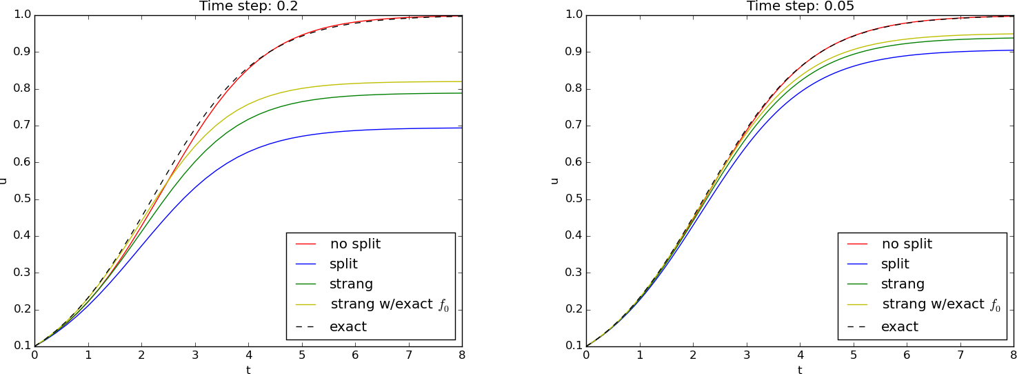
Figure 79 shows that the impact of splitting is significant. Interestingly, however, the Forward Euler method applied to the entire problem directly is much more accurate than any of the splitting schemes. We also see that Strang splitting is definitely more accurate than ordinary splitting and that it helps a bit to use an exact solution of \( u'=f_0(u) \). With a large time step (\( \Delta t = 0.2 \), left plot in Figure 79), the asymptotic values are off by 20-30%. A more reasonable time step (\( \Delta t = 0.05 \), right plot in Figure 79) gives better results, but still the asymptotic values are up to 10% wrong.
As technique for solving nonlinear ODEs, we realize that the present case study is not particularly promising, as the Forward Euler method both linearizes the original problem and provides a solution that is much more accurate than any of the splitting techniques. In complicated multi-physics settings, on the other hand, splitting may be the only feasible way to go, and sometimes you really need to apply different numerics to different parts of a PDE problem. But in very simple problems, like the logistic ODE, splitting is just an inferior technique. Still, the logistic ODE is ideal for introducing all the mathematical details and for investigating the behavior.
Figure 79: Effect of ordinary and Strang splitting for the logistic equation.
Reaction-diffusion equation
Consider a diffusion equation coupled to chemical reactions modeled by a nonlinear term \( f(u) \): $$ \frac{\partial u}{\partial t} = \dfc\nabla^2u + f(u)\tp$$ This is a physical process composed of two individual processes: \( u \) is the concentration of a substance that is locally generated by a chemical reaction \( f(u) \), while \( u \) is spreading in space because of diffusion. There are obviously two time scales: one for the chemical reaction and one for diffusion. Typically, fast chemical reactions require much finer time stepping than slower diffusion processes. It could therefore be advantageous to split the two physical effects in separate models and use different numerical methods for the two.
A natural spitting in the present case is $$ \begin{align} \frac{\partial u^{\stepzero}}{\partial t} &= \dfc\nabla^2 u^{\stepzero}, \tag{5.79}\\ \frac{\partial u^{\stepone}}{\partial t} &= f(u^{\stepone}) \tag{5.80}\tp \end{align} $$ Looking at these familiar problems, we may apply a \( \theta \) rule (implicit) scheme for (5.79) over one time step and avoid dealing with nonlinearities by applying an explicit scheme for (5.80) over the same time step.
Suppose we have some solution \( u \) at time level \( t_n \). For flexibility, we define a \( \theta \) method for the diffusion part (5.79) by $$ [D_t u^\stepzero = \dfc (D_xD_x u^\stepzero + D_y D_y u^\stepzero)]^{n+\theta}\tp$$ We use \( u^{n} \) as initial condition for \( u^\stepzero \).
The reaction part, which is defined at each mesh point (without coupling values in different mesh points), can employ any scheme for an ODE. Here we use an Adams-Bashforth method of order 2. Recall that the overall accuracy of the splitting method is maximum \( \Oof{\Delta t^2} \) for Strang splitting, otherwise it is just \( \Oof{\Delta t} \). Higher-order methods for ODEs will therefore be a waste of work. The 2nd-order Adams-Bashforth method reads $$ \begin{equation} u^{\stepone,n+1}_{i,j} = u^{\stepone,n}_{i,j} + \half\Delta t\left( 3f(u^{\stepone, n}_{i,j}, t_n) - f(u^{\stepone, n-1}_{i,j}, t_{n-1}) \right) \tp \tag{5.81} \end{equation} $$ We can use a Forward Euler step to start the method, i.e, compute \( u^{\stepone,1}_{i,j} \).
The algorithm goes like this:
- Solve the diffusion problem for one time step as usual.
- Solve the reaction ODEs at each mesh point in \( [t_n,t_n+\Delta t] \), using the diffusion solution in 1. as initial condition. The solution of the ODEs constitute the solution of the original problem at the end of each time step.
Example: Reaction-Diffusion with linear reaction term
The methods above may be explored in detail through a specific computational example in which we compute the convergence rates associated with four different solution approaches for the reaction-diffusion equation with a linear reaction term, i.e. \( f(u)=-bu \). The methods comprise solving without splitting (just straight forward Euler), ordinary splitting, first order Strang splitting, and second order Strang splitting. In all four methods, a standard centered difference approximation is used for the spatial second derivative. The methods share the error model \( E = C h^r \), while differing in the step \( h \) (being either \( dx^2 \) or \( dx \)) and the convergence rate \( r \) (being either 1 or 2).
All code commented below is found in the file
split_diffu_react.py. When executed,
a function convergence_rates is called, from which all convergence
rate computations are handled:
def convergence_rates(scheme='diffusion'):

    F = 0.5
    T = 1.2
    a = 3.5
    b = 1
    L = 1.5
    k = np.pi/L

    def exact(x, t):
        '''exact sol. to: du/dt = a*d^2u/dx^2 - b*u'''
        return np.exp(-(a*k**2 + b)*t) * np.sin(k*x)

    def f(u, t):
        return -b*u

    def I(x):
        return exact(x, 0)

    global error    # error computed in the user action function
    error = 0

    # Convergence study
    def action(u, x, t, n):
        global error
        if n == 1:      # New simulation, - reset error
            error = 0
        else:
            error = max(error, np.abs(u - exact(x, t[n])).max())

    E = []
    h = []
    Nx_values = [10, 20, 40, 80]
    for Nx in Nx_values:
        dx = L/Nx
        dt = F/a*dx**2
        Nt = int(round(T/float(dt)))
        t = np.linspace(0, Nt*dt, Nt+1)   # Mesh points, global time

        if scheme == 'diffusion':
            print 'Running FE on whole eqn...'
            diffusion_theta(I, a, f, L, dt, F, t, T,
                            step_no=0, theta=0,
                            u_L=0, u_R=0, user_action=action)
            h.append(dx**2)
        elif scheme == 'ordinary_splitting':
            print 'Running ordinary splitting...'
            ordinary_splitting(I=I, a=a, b=b, f=f, L=L, dt=dt,
                               dt_Rfactor=1, F=F, t=t, T=T,
                               user_action=action)
            h.append(dx**2)
        elif scheme == 'Strang_splitting_1stOrder':
            print 'Running Strang splitting with 1st order schemes...'
            Strang_splitting_1stOrder(I=I, a=a, b=b, f=f, L=L, dt=dt,
                                      dt_Rfactor=1, F=F, t=t, T=T,
                                      user_action=action)
            h.append(dx**2)
        elif scheme == 'Strang_splitting_2ndOrder':
            print 'Running Strang splitting with 2nd order schemes...'
            Strang_splitting_2ndOrder(I=I, a=a, b=b, f=f, L=L, dt=dt,
                                      dt_Rfactor=1, F=F, t=t, T=T,
                                      user_action=action)
            h.append(dx)
        else:
            print 'Unknown scheme requested!'
            sys.exit(0)

        E.append(error)

    print 'E:', E
    print 'h:', h

    # Convergence rates
    r = [np.log(E[i]/E[i-1])/np.log(h[i]/h[i-1])
         for i in range(1,len(Nx_values))]
    print 'Computed rates:', r


if __name__ == '__main__':

    schemes = ['diffusion',
               'ordinary_splitting',
               'Strang_splitting_1stOrder',
               'Strang_splitting_2ndOrder']

    for scheme in schemes:
        convergence_rates(scheme=scheme)
The Fourier number is kept fixed throughout at \( F = 0.5 \), being the stability
limit with explicit schemes. Since \( \alpha \) is considered a known constant and
\( F = \frac{\alpha dt}{dx^2} \), \( dt \) (or \( dx \)) is readily computed
for a given \( dx \) (or \( dt \)). The loop in convergence_rates runs over a chosen
set of grid points implying a doubling of spatial resolution with each iteration.
A solver diffusion_theta is used in each of the four solution approaches:
def diffusion_theta(I, a, f, L, dt, F, t, T, step_no, theta=0.5,
                    u_L=0, u_R=0, user_action=None):
    """
    Full solver for the model problem using the theta-rule
    difference approximation in time (no restriction on F,
    i.e., the time step when theta >= 0.5).     Vectorized
    implementation and sparse (tridiagonal) coefficient matrix.
    Note that t always covers the whole global time interval, whether
    splitting is the case or not. T, on the other hand, is
    the end of the global time interval if there is no split,
    but if splitting, we use T=dt. When splitting, step_no
    keeps track of the time step number (for lookup in t).
    """

    Nt = int(round(T/float(dt)))
    dx = np.sqrt(a*dt/F)
    Nx = int(round(L/dx))
    x = np.linspace(0, L, Nx+1)       # Mesh points in space
    # Make sure dx and dt are compatible with x and t
    dx = x[1] - x[0]
    dt = t[1] - t[0]

    u   = np.zeros(Nx+1)   # solution array at t[n+1]
    u_1 = np.zeros(Nx+1)   # solution at t[n]

    # Representation of sparse matrix and right-hand side
    diagonal = np.zeros(Nx+1)
    lower    = np.zeros(Nx)
    upper    = np.zeros(Nx)
    b        = np.zeros(Nx+1)

    # Precompute sparse matrix (scipy format)
    Fl = F*theta
    Fr = F*(1-theta)
    diagonal[:] = 1 + 2*Fl
    lower[:] = -Fl  #1
    upper[:] = -Fl  #1
    # Insert boundary conditions
    diagonal[0] = 1
    upper[0] = 0
    diagonal[Nx] = 1
    lower[-1] = 0

    diags = [0, -1, 1]
    A = scipy.sparse.diags(
        diagonals=[diagonal, lower, upper],
        offsets=[0, -1, 1], shape=(Nx+1, Nx+1),
        format='csr')
    #print A.todense()

    # Allow f to be None or 0
    if f is None or f == 0:
        f = lambda x, t: np.zeros((x.size)) \
            if isinstance(x, np.ndarray) else 0

    # Set initial condition
    if isinstance(I, np.ndarray):   # I is an array
        u_1 = np.copy(I)
    else:                           # I is a function
        for i in range(0, Nx+1):
            u_1[i] = I(x[i])

    if user_action is not None:
        user_action(u_1, x, t, step_no+0)

    # Time loop
    for n in range(0, Nt):
        b[1:-1] = u_1[1:-1] + \
                  Fr*(u_1[:-2] - 2*u_1[1:-1] + u_1[2:]) + \
                  dt*theta*f(u_1[1:-1], t[step_no+n+1]) + \
                  dt*(1-theta)*f(u_1[1:-1], t[step_no+n])
        b[0] = u_L; b[-1] = u_R  # boundary conditions
        u[:] = scipy.sparse.linalg.spsolve(A, b)

        if user_action is not None:
            user_action(u, x, t, step_no+(n+1))

        # Update u_1 before next step
        u_1, u = u, u_1

    # u is now contained in u_1 (swapping)
    return u_1
For the no splitting approach with forward Euler in time, this solver handles both
the diffusion and the reaction term. When splitting, diffusion_theta takes care
of the diffusion term only, while the reaction
term is handled either by a forward Euler scheme in reaction_FE, or by a
second order Adams-Bashforth scheme from Odespy. The reaction_FE function
covers one complete time step dt during ordinary splitting, while Strang
splitting (both first and second order) applies it with dt/2 twice during
each time step dt. Since the reaction term typically represents a much faster
process than the diffusion term, a further refinement of the time step is made
possible in reaction_FE. It was implemented as
def reaction_FE(I, f, L, Nx, dt, dt_Rfactor, t, step_no,
                user_action=None):
    """Reaction solver, Forward Euler method.
    Note the at t covers the whole global time interval.
    dt is either one complete,or one half, of the step in the
    diffusion part, i.e. there is a local time interval
    [0, dt] or [0, dt/2] that the reaction_FE
    deals with each time it is called. step_no keeps
    track of the (global) time step number (required
    for lookup in t).
    """

    u = np.copy(I)
    dt_local = dt/float(dt_Rfactor)
    Nt_local = int(round(dt/float(dt_local)))
    x = np.linspace(0, L, Nx+1)

    for n in range(Nt_local):
        time = t[step_no] + n*dt_local
        u[1:Nx] = u[1:Nx] + dt_local*f(u[1:Nx], time)

    # BC already inserted in diffusion step, i.e. no action here
    return u
With the ordinary splitting approach, each time step dt is covered twice. First
computing the impact of the reaction term, then the contribution from the diffusion term:
def ordinary_splitting(I, a, b, f, L, dt,
                       dt_Rfactor, F, t, T,
                       user_action=None):
    '''1st order scheme, i.e. Forward Euler is enough for both
    the diffusion and the reaction part. The time step dt is
    given for the diffusion step, while the time step for the
    reaction part is found as dt/dt_Rfactor, where dt_Rfactor >= 1.
    '''
    Nt = int(round(T/float(dt)))
    dx = np.sqrt(a*dt/F)
    Nx = int(round(L/dx))
    x = np.linspace(0, L, Nx+1)       # Mesh points in space
    u = np.zeros(Nx+1)

    # Set initial condition u(x,0) = I(x)
    for i in range(0, Nx+1):
        u[i] = I(x[i])

    # In the following loop, each time step is "covered twice",
    # first for reaction, then for diffusion
    for n in range(0, Nt):
        # Reaction step (potentially many smaller steps within dt)
        u_s = reaction_FE(I=u, f=f, L=L, Nx=Nx,
                        dt=dt, dt_Rfactor=dt_Rfactor,
                        t=t, step_no=n,
                        user_action=None)

        u = diffusion_theta(I=u_s, a=a, f=0, L=L, dt=dt, F=F,
                              t=t, T=dt, step_no=n, theta=0,
                              u_L=0, u_R=0, user_action=None)

        if user_action is not None:
            user_action(u, x, t, n+1)

    return
For the two Strang splitting approaches, each time step dt is handled by first computing
the reaction step for (the first) dt/2, followed by a diffusion step dt, before the reaction step
is treated once again for (the remaining) dt/2. Since first order Strang splitting is no better than first order accurate, both the reaction and diffusion steps are computed explicitly. The
solver was implemented as
def Strang_splitting_1stOrder(I, a, b, f, L, dt, dt_Rfactor,
                              F, t, T, user_action=None):
    '''Strang splitting while still using FE for the reaction
    step and for the diffusion step. Gives 1st order scheme.
    The time step dt is given for the diffusion step, while
    the time step for the reaction part is found as
    0.5*dt/dt_Rfactor, where dt_Rfactor >= 1. Introduce an
    extra time mesh t2 for the reaction part, since it steps dt/2.
    '''
    Nt = int(round(T/float(dt)))
    t2 = np.linspace(0, Nt*dt, (Nt+1)+Nt)   # Mesh points in diff
    dx = np.sqrt(a*dt/F)
    Nx = int(round(L/dx))
    x = np.linspace(0, L, Nx+1)
    u = np.zeros(Nx+1)

    # Set initial condition u(x,0) = I(x)
    for i in range(0, Nx+1):
        u[i] = I(x[i])

    for n in range(0, Nt):
        # Reaction step (1/2 dt: from t_n to t_n+1/2)
        # (potentially many smaller steps within dt/2)
        u_s = reaction_FE(I=u, f=f, L=L, Nx=Nx,
                        dt=dt/2.0, dt_Rfactor=dt_Rfactor,
                        t=t2, step_no=2*n,
                        user_action=None)
        # Diffusion step (1 dt: from t_n to t_n+1)
        u_sss = diffusion_theta(I=u_s, a=a, f=0, L=L, dt=dt, F=F,
                              t=t, T=dt, step_no=n, theta=0,
                              u_L=0, u_R=0, user_action=None)
        # Reaction step (1/2 dt: from t_n+1/2 to t_n+1)
        # (potentially many smaller steps within dt/2)
        u = reaction_FE(I=u_sss, f=f, L=L, Nx=Nx,
                        dt=dt/2.0, dt_Rfactor=dt_Rfactor,
                        t=t2, step_no=2*n+1,
                        user_action=None)

        if user_action is not None:
            user_action(u, x, t, n+1)

    return
The second order version of the Strang splitting approach utilizes a second order Adams-Bashforth solver for the reaction part and a Crank-Nicolson scheme for the diffusion part. The solver has the same structure as the one for first order Strang splitting and was implemented as
def Strang_splitting_2ndOrder(I, a, b, f, L, dt, dt_Rfactor,
                              F, t, T, user_action=None):
    '''Strang splitting using Crank-Nicolson for the diffusion
    step (theta-rule) and Adams-Bashforth 2 for the reaction step.
    Gives 2nd order scheme. Introduce an extra time mesh t2 for
    the reaction part, since it steps dt/2.
    '''
    import odespy
    Nt = int(round(T/float(dt)))
    t2 = np.linspace(0, Nt*dt, (Nt+1)+Nt)   # Mesh points in diff
    dx = np.sqrt(a*dt/F)
    Nx = int(round(L/dx))
    x = np.linspace(0, L, Nx+1)
    u = np.zeros(Nx+1)

    # Set initial condition u(x,0) = I(x)
    for i in range(0, Nx+1):
        u[i] = I(x[i])

    reaction_solver = odespy.AdamsBashforth2(f)

    for n in range(0, Nt):
        # Reaction step (1/2 dt: from t_n to t_n+1/2)
        # (potentially many smaller steps within dt/2)
        reaction_solver.set_initial_condition(u)
        t_points = np.linspace(0, dt/2.0, dt_Rfactor+1)
        u_AB2, t_ = reaction_solver.solve(t_points) # t_ not needed
        u_s = u_AB2[-1,:]  # pick sol at last point in time

        # Diffusion step (1 dt: from t_n to t_n+1)
        u_sss = diffusion_theta(I=u_s, a=a, f=0, L=L, dt=dt, F=F,
                              t=t, T=dt, step_no=n, theta=0.5,
                              u_L=0, u_R=0, user_action=None)
        # Reaction step (1/2 dt: from t_n+1/2 to t_n+1)
        # (potentially many smaller steps within dt/2)
        reaction_solver.set_initial_condition(u_sss)
        t_points = np.linspace(0, dt/2.0, dt_Rfactor+1)
        u_AB2, t_ = reaction_solver.solve(t_points) # t_ not needed
        u = u_AB2[-1,:]  # pick sol at last point in time

        if user_action is not None:
            user_action(u, x, t, n+1)

    return
When executing split_diffu_react.py, we find that the estimated convergence rates
are as expected. The second order Strang splitting has second order convergence (\( r = 2 \)), while
the remaining three approaches have first order convergence (\( r = 1 \)).
Analysis of the splitting method
Let us address a linear PDE problem for which we can develop analytical solutions of the discrete equations, with and without splitting, and discuss these. Choosing \( f(u)=-\beta u \) for a constant \( \beta \) gives a linear problem. We use the Forward Euler method for both the PDE and ODE problems.
We seek a 1D Fourier wave component solution of the problem, assuming homogeneous Dirichlet conditions at \( x=0 \) and \( x=L \): $$ u = e^{-\dfc k^2 t - \beta t}\sin kx,\quad k = \frac{\pi}{L}\tp$$ This component fits the 1D PDE problem (\( f=0 \)). On complex form we can write $$ u = e^{-\dfc k^2 t - \beta t + ikx},$$ where \( i=\sqrt{-1} \) and the imaginary part is taken as the physical solution.
We refer to the section Analysis of schemes for the diffusion equation and to the book [2] for a discussion of exact numerical solutions to diffusion and decay problems, respectively. The key idea is to search for solutions \( A^ne^{ikx} \) and determine \( A \). For the diffusion problem solved by a Forward Euler method one has $$ A = 1 - 4F\sin^p, $$ where \( F=\dfc\Delta t/\Delta x^2 \) is the mesh Fourier number and \( p=k\Delta x/2 \) is a dimensionless number reflecting the spatial resolution (number of points per wave length in space). For the decay problem \( u'=-\beta u \), we have \( A=1 - q \), where \( q \) is a dimensionless parameter reflecting the resolution in the decay problem: \( q = \beta\Delta t \).
The original model problem can also be discretized by a Forward Euler scheme, $$ [D^+_t u = \dfc D_xD_x u - \beta u]^n_i\tp$$ Assuming \( A^ne^{ikx} \) we find that $$ u^n_i = (1 - 4F\sin^p -q)^n\sin kx\tp$$ We are particularly interested in what happens at one time step. That is, $$ u^{n}_{i} = (1-4F\sin^2 p)u^{n-1}_i\tp$$
In the two stage algorithm, we first compute the diffusion step $$ u^{\stepzero,n+1}_i = (1 - 4F\sin^2 p)u^{n-1}_i\tp$$ Then we use this as input to the decay algorithm and arrive at $$ u^{\stepone,n+1} = (1-q)u^{\stepzero,n+1} = (1-q)(1-4F\sin^2 p) u^{n-1}_i\tp$$ The splitting approximation over one step is therefore $$ E = 1 - 4F\sin^p -q - (1-q)(1-4F\sin^2 p) = -q(2 - F\sin^2 p)) $$