Generalization: damping, nonlinearities, and excitation

We shall now generalize the simple model problem from the section Finite difference discretization to include a possibly nonlinear damping term \( f(u^{\prime}) \), a possibly nonlinear spring (or restoring) force \( s(u) \), and some external excitation \( F(t) \): $$ \begin{equation} mu^{\prime\prime} + f(u^{\prime}) + s(u) = F(t),\quad u(0)=I,\ u^{\prime}(0)=V,\ t\in (0,T] \tp \tag{1.71} \end{equation} $$ We have also included a possibly nonzero initial value of \( u^{\prime}(0) \). The parameters \( m \), \( f(u^{\prime}) \), \( s(u) \), \( F(t) \), \( I \), \( V \), and \( T \) are input data.

There are two main types of damping (friction) forces: linear \( f(u^{\prime})=bu \), or quadratic \( f(u^{\prime})=bu^{\prime}|u^{\prime}| \). Spring systems often feature linear damping, while air resistance usually gives rise to quadratic damping. Spring forces are often linear: \( s(u)=cu \), but nonlinear versions are also common, the most famous is the gravity force on a pendulum that acts as a spring with \( s(u)\sim \sin(u) \).

A centered scheme for linear damping

Sampling (1.71) at a mesh point \( t_n \), replacing \( u^{\prime\prime}(t_n) \) by \( [D_tD_tu]^n \), and \( u^{\prime}(t_n) \) by \( [D_{2t}u]^n \) results in the discretization $$ \begin{equation} [mD_tD_t u + f(D_{2t}u) + s(u) = F]^n, \tag{1.72} \end{equation} $$ which written out means $$ \begin{equation} m\frac{u^{n+1}-2u^n + u^{n-1}}{\Delta t^2} + f(\frac{u^{n+1}-u^{n-1}}{2\Delta t}) + s(u^n) = F^n, \tag{1.73} \end{equation} $$ where \( F^n \) as usual means \( F(t) \) evaluated at \( t=t_n \). Solving (1.73) with respect to the unknown \( u^{n+1} \) gives a problem: the \( u^{n+1} \) inside the \( f \) function makes the equation nonlinear unless \( f(u^{\prime}) \) is a linear function, \( f(u^{\prime})=bu^{\prime} \). For now we shall assume that \( f \) is linear in \( u^{\prime} \). Then $$ \begin{equation} m\frac{u^{n+1}-2u^n + u^{n-1}}{\Delta t^2} + b\frac{u^{n+1}-u^{n-1}}{2\Delta t} + s(u^n) = F^n, \tag{1.74} \end{equation} $$ which gives an explicit formula for \( u \) at each new time level: $$ \begin{equation} u^{n+1} = (2mu^n + (\frac{b}{2}\Delta t - m)u^{n-1} + \Delta t^2(F^n - s(u^n)))(m + \frac{b}{2}\Delta t)^{-1} \tag{1.75} \tp \end{equation} $$

For the first time step we need to discretize \( u^{\prime}(0)=V \) as \( [D_{2t}u = V]^0 \) and combine with (1.75) for \( n=0 \). The discretized initial condition leads to $$ \begin{equation} u^{-1} = u^{1} - 2\Delta t V, \tag{1.76} \end{equation} $$ which inserted in (1.75) for \( n=0 \) gives an equation that can be solved for \( u^1 \): $$ \begin{equation} u^1 = u^0 + \Delta t\, V + \frac{\Delta t^2}{2m}(-bV - s(u^0) + F^0) \tp \tag{1.77} \end{equation} $$

A centered scheme for quadratic damping

When \( f(u^{\prime})=bu^{\prime}|u^{\prime}| \), we get a quadratic equation for \( u^{n+1} \) in (1.73). This equation can be straightforwardly solved by the well-known formula for the roots of a quadratic equation. However, we can also avoid the nonlinearity by introducing an approximation with an error of order no higher than what we already have from replacing derivatives with finite differences.

We start with (1.71) and only replace \( u^{\prime\prime} \) by \( D_tD_tu \), resulting in $$ \begin{equation} [mD_tD_t u + bu^{\prime}|u^{\prime}| + s(u) = F]^n\tp \tag{1.78} \end{equation} $$ Here, \( u^{\prime}|u^{\prime}| \) is to be computed at time \( t_n \). The idea is now to introduce a geometric mean, defined by $$ (w^2)^n \approx w^{n-\half}w^{n+\half},$$ for some quantity \( w \) depending on time. The error in the geometric mean approximation is \( \Oof{\Delta t^2} \), the same as in the approximation \( u^{\prime\prime}\approx D_tD_tu \). With \( w=u^{\prime} \) it follows that $$ [u^{\prime}|u^{\prime}|]^n \approx u^{\prime}(t_{n+\half})|u^{\prime}(t_{n-\half})|\tp$$ The next step is to approximate \( u^{\prime} \) at \( t_{n\pm 1/2} \), and fortunately a centered difference fits perfectly into the formulas since it involves \( u \) values at the mesh points only. With the approximations $$ \begin{equation} u^{\prime}(t_{n+1/2})\approx [D_t u]^{n+\half},\quad u^{\prime}(t_{n-1/2})\approx [D_t u]^{n-\half}, \tag{1.79} \end{equation} $$ we get $$ \begin{equation} [u^{\prime}|u^{\prime}|]^n \approx [D_tu]^{n+\half}|[D_tu]^{n-\half}| = \frac{u^{n+1}-u^n}{\Delta t} \frac{|u^n-u^{n-1}|}{\Delta t} \tp \tag{1.80} \end{equation} $$ The counterpart to (1.73) is then $$ \begin{equation} m\frac{u^{n+1}-2u^n + u^{n-1}}{\Delta t^2} + b\frac{u^{n+1}-u^n}{\Delta t}\frac{|u^n-u^{n-1}|}{\Delta t} + s(u^n) = F^n, \tag{1.81} \end{equation} $$ which is linear in the unknown \( u^{n+1} \). Therefore, we can easily solve (1.81) with respect to \( u^{n+1} \) and achieve the explicit updating formula $$ \begin{align} u^{n+1} &= \left( m + b|u^n-u^{n-1}|\right)^{-1}\times \nonumber\\ & \qquad \left(2m u^n - mu^{n-1} + bu^n|u^n-u^{n-1}| + \Delta t^2 (F^n - s(u^n)) \right) \tp \tag{1.82} \end{align} $$

In the derivation of a special equation for the first time step we run into some trouble: inserting (1.76) in (1.82) for \( n=0 \) results in a complicated nonlinear equation for \( u^1 \). By thinking differently about the problem we can easily get away with the nonlinearity again. We have for \( n=0 \) that \( b[u^{\prime}|u^{\prime}|]^0 = bV|V| \). Using this value in (1.78) gives $$ \begin{equation} [mD_tD_t u + bV|V| + s(u) = F]^0 \tp \tag{1.83} \end{equation} $$ Writing this equation out and using (1.76) results in the special equation for the first time step: $$ \begin{equation} u^1 = u^0 + \Delta t V + \frac{\Delta t^2}{2m}\left(-bV|V| - s(u^0) + F^0\right) \tp \tag{1.84} \end{equation} $$

A forward-backward discretization of the quadratic damping term

The previous section first proposed to discretize the quadratic damping term \( |u^{\prime}|u^{\prime} \) using centered differences: \( [|D_{2t}|D_{2t}u]^n \). As this gives rise to a nonlinearity in \( u^{n+1} \), it was instead proposed to use a geometric mean combined with centered differences. But there are other alternatives. To get rid of the nonlinearity in \( [|D_{2t}|D_{2t}u]^n \), one can think differently: apply a backward difference to \( |u^{\prime}| \), such that the term involves known values, and apply a forward difference to \( u^{\prime} \) to make the term linear in the unknown \( u^{n+1} \). With mathematics, $$ \begin{equation} [\beta |u^{\prime}|u^{\prime}]^n \approx \beta |[D_t^-u]^n|[D_t^+ u]^n = \beta\left\vert\frac{u^n-u^{n-1}}{\Delta t}\right\vert \frac{u^{n+1}-u^n}{\Delta t}\tp \tag{1.85} \end{equation} $$ The forward and backward differences have both an error proportional to \( \Delta t \) so one may think the discretization above leads to a first-order scheme. However, by looking at the formulas, we realize that the forward-backward differences in (1.85) result in exactly the same scheme as in (1.81) where we used a geometric mean and centered differences and committed errors of size \( \Oof{\Delta t^2} \). Therefore, the forward-backward differences in (1.85) act in a symmetric way and actually produce a second-order accurate discretization of the quadratic damping term.

Implementation

The algorithm arising from the methods in the sections A centered scheme for linear damping and A centered scheme for quadratic damping is very similar to the undamped case in the section A centered finite difference scheme. The difference is basically a question of different formulas for \( u^1 \) and \( u^{n+1} \). This is actually quite remarkable. The equation (1.71) is normally impossible to solve by pen and paper, but possible for some special choices of \( F \), \( s \), and \( f \). On the contrary, the complexity of the nonlinear generalized model (1.71) versus the simple undamped model is not a big deal when we solve the problem numerically!

The computational algorithm takes the form

1. \( u^0=I \)
2. compute \( u^1 \) from (1.77) if linear damping or (1.84) if quadratic damping
3. for \( n=1,2,\ldots,N_t-1 \):
   1. compute \( u^{n+1} \) from (1.75) if linear damping or (1.82) if quadratic damping

def solver(I, V, m, b, s, F, dt, T, damping='linear'):
    """
    Solve m*u'' + f(u') + s(u) = F(t) for t in (0,T],
    u(0)=I and u'(0)=V,
    by a central finite difference method with time step dt.
    If damping is 'linear', f(u')=b*u, while if damping is
    'quadratic', f(u')=b*u'*abs(u').
    F(t) and s(u) are Python functions.
    """
    dt = float(dt); b = float(b); m = float(m) # avoid integer div.
    Nt = int(round(T/dt))
    u = np.zeros(Nt+1)
    t = np.linspace(0, Nt*dt, Nt+1)

    u[0] = I
    if damping == 'linear':
        u[1] = u[0] + dt*V + dt**2/(2*m)*(-b*V - s(u[0]) + F(t[0]))
    elif damping == 'quadratic':
        u[1] = u[0] + dt*V + \ 
               dt**2/(2*m)*(-b*V*abs(V) - s(u[0]) + F(t[0]))

    for n in range(1, Nt):
        if damping == 'linear':
            u[n+1] = (2*m*u[n] + (b*dt/2 - m)*u[n-1] +
                      dt**2*(F(t[n]) - s(u[n])))/(m + b*dt/2)
        elif damping == 'quadratic':
            u[n+1] = (2*m*u[n] - m*u[n-1] + b*u[n]*abs(u[n] - u[n-1])
                      + dt**2*(F(t[n]) - s(u[n])))/\ 
                      (m + b*abs(u[n] - u[n-1]))
    return u, t

The complete code resides in the file vib.py.

Verification

Constant solution

For debugging and initial verification, a constant solution is often very useful. We choose \( \uex(t)=I \), which implies \( V=0 \). Inserted in the ODE, we get \( F(t)=s(I) \) for any choice of \( f \). Since the discrete derivative of a constant vanishes (in particular, \( [D_{2t}I]^n=0 \), \( [D_tI]^n=0 \), and \( [D_tD_t I]^n=0 \)), the constant solution also fulfills the discrete equations. The constant should therefore be reproduced to machine precision. The function test_constant in vib.py implements this test.

Linear solution

Now we choose a linear solution: \( \uex = ct + d \). The initial condition \( u(0)=I \) implies \( d=I \), and \( u^{\prime}(0)=V \) forces \( c \) to be \( V \). Inserting \( \uex=Vt+I \) in the ODE with linear damping results in $$ 0 + bV + s(Vt+I) = F(t),$$ while quadratic damping requires the source term $$ 0 + b|V|V + s(Vt+I) = F(t)\tp$$ Since the finite difference approximations used to compute \( u^{\prime} \) all are exact for a linear function, it turns out that the linear \( \uex \) is also a solution of the discrete equations. Exercise 1.10: Use linear/quadratic functions for verification asks you to carry out all the details.

Quadratic solution

Choosing \( \uex = bt^2 + Vt + I \), with \( b \) arbitrary, fulfills the initial conditions and fits the ODE if \( F \) is adjusted properly. The solution also solves the discrete equations with linear damping. However, this quadratic polynomial in \( t \) does not fulfill the discrete equations in case of quadratic damping, because the geometric mean used in the approximation of this term introduces an error. Doing Exercise 1.10: Use linear/quadratic functions for verification will reveal the details. One can fit \( F^n \) in the discrete equations such that the quadratic polynomial is reproduced by the numerical method (to machine precision).

Catching bugs

How good are the constant and quadratic solutions at catching bugs in the implementation?

• Use m instead of 2*m in the denominator of u[1]: constant works, while quadratic fails.
• Use b*dt instead of b*dt/2 in the updating formula for u[n+1] in case of linear damping: constant and quadratic fail.
• Use F[n+1] instead of F[n] in case of linear or quadratic damping: constant solution works, quadratic fails.

Visualization

The functions for visualizations differ significantly from those in the undamped case in the vib_undamped.py program because, in the present general case, we do not have an exact solution to include in the plots. Moreover, we have no good estimate of the periods of the oscillations as there will be one period determined by the system parameters, essentially the approximate frequency \( \sqrt{s'(0)/m} \) for linear \( s \) and small damping, and one period dictated by \( F(t) \) in case the excitation is periodic. This is, however, nothing that the program can depend on or make use of. Therefore, the user has to specify \( T \) and the window width to get a plot that moves with the graph and shows the most recent parts of it in long time simulations.

The vib.py code contains several functions for analyzing the time series signal and for visualizing the solutions.

User interface

The main function is changed substantially from the vib_undamped.py code, since we need to specify the new data \( c \), \( s(u) \), and \( F(t) \). In addition, we must set \( T \) and the plot window width (instead of the number of periods we want to simulate as in vib_undamped.py). To figure out whether we can use one plot for the whole time series or if we should follow the most recent part of \( u \), we can use the plot_empricial_freq_and_amplitude function's estimate of the number of local maxima. This number is now returned from the function and used in main to decide on the visualization technique.

def main():
    import argparse
    parser = argparse.ArgumentParser()
    parser.add_argument('--I', type=float, default=1.0)
    parser.add_argument('--V', type=float, default=0.0)
    parser.add_argument('--m', type=float, default=1.0)
    parser.add_argument('--c', type=float, default=0.0)
    parser.add_argument('--s', type=str, default='u')
    parser.add_argument('--F', type=str, default='0')
    parser.add_argument('--dt', type=float, default=0.05)
    parser.add_argument('--T', type=float, default=140)
    parser.add_argument('--damping', type=str, default='linear')
    parser.add_argument('--window_width', type=float, default=30)
    parser.add_argument('--savefig', action='store_true')
    a = parser.parse_args()
    from scitools.std import StringFunction
    s = StringFunction(a.s, independent_variable='u')
    F = StringFunction(a.F, independent_variable='t')
    I, V, m, c, dt, T, window_width, savefig, damping = \ 
       a.I, a.V, a.m, a.c, a.dt, a.T, a.window_width, a.savefig, \ 
       a.damping

    u, t = solver(I, V, m, c, s, F, dt, T)
    num_periods = empirical_freq_and_amplitude(u, t)
    if num_periods <= 15:
        figure()
        visualize(u, t)
    else:
        visualize_front(u, t, window_width, savefig)
    show()

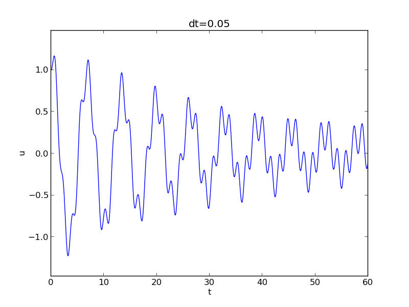
The program vib.py contains the above code snippets and can solve the model problem (1.71). As a demo of vib.py, we consider the case \( I=1 \), \( V=0 \), \( m=1 \), \( c=0.03 \), \( s(u)=\sin(u) \), \( F(t)=3\cos(4t) \), \( \Delta t = 0.05 \), and \( T=140 \). The relevant command to run is

Terminal> python vib.py --s 'sin(u)' --F '3*cos(4*t)' --c 0.03

This results in a moving window following the function on the screen. Figure 17 shows a part of the time series.

The Euler-Cromer scheme for the generalized model

The ideas of the Euler-Cromer method from the section The Euler-Cromer method carry over to the generalized model. We write (1.71) as two equations for \( u \) and \( v=u^{\prime} \). The first equation is taken as the one with \( v^{\prime} \) on the left-hand side: $$ \begin{align} v^{\prime} &= \frac{1}{m}(F(t)-s(u)-f(v)), \tag{1.86}\\ u^{\prime} &= v\tp \tag{1.87} \end{align} $$ The idea is to step (1.86) forward using a standard Forward Euler method, while we update \( u \) from (1.87) with a Backward Euler method, utilizing the recent, computed \( v^{n+1} \) value. In detail, $$ \begin{align} \frac{v^{n+1}-v^n}{\Delta t} &= \frac{1}{m}(F(t_n)-s(u^n)-f(v^n)), \tag{1.88}\\ \frac{u^{n+1}-u^n}{\Delta t} &= v^{n+1}, \tag{1.89} \end{align} $$ resulting in the explicit scheme $$ \begin{align} v^{n+1} &= v^n + \Delta t\frac{1}{m}(F(t_n)-s(u^n)-f(v^n)), \tag{1.90}\\ u^{n+1} &= u^n + \Delta t\,v^{n+1}\tp \tag{1.91} \end{align} $$ We immediately note one very favorable feature of this scheme: all the nonlinearities in \( s(u) \) and \( f(v) \) are evaluated at a previous time level. This makes the Euler-Cromer method easier to apply and hence much more convenient than the centered scheme for the second-order ODE (1.71).

The initial conditions are trivially set as $$ \begin{align} v^0 &= V, \tag{1.92}\\ u^0 &= I\tp \tag{1.93} \end{align} $$

The Stoermer-Verlet algorithm for the generalized model

We can easily apply the ideas from the section The Stoermer-Verlet algorithm to extend that method to the generalized model $$ \begin{align*} v^{\prime} &= \frac{1}{m}(F(t)-s(u)-f(v)),\\ u^{\prime} &= v\tp \end{align*} $$ However, since the scheme is essentially centered differences for the ODE system on a staggered mesh, we do not go into detail here, but refer to the section A staggered Euler-Cromer scheme for a generalized model.

A staggered Euler-Cromer scheme for a generalized model

The more general model for vibration problems, $$ \begin{equation} mu'' + f(u') + s(u) = F(t),\quad u(0)=I,\ u'(0)=V,\ t\in (0,T], \tag{1.94} \end{equation} $$ can be rewritten as a first-order ODE system $$ \begin{align} v' &= m^{-1}\left(F(t) - f(v) - s(u)\right), \tag{1.95}\\ u' &= v\tp \tag{1.96} \end{align} $$ It is natural to introduce a staggered mesh (see the section The Euler-Cromer scheme on a staggered mesh) and seek \( u \) at mesh points \( t_n \) (the numerical value is denoted by \( u^n \)) and \( v \) between mesh points at \( t_{n+1/2} \) (the numerical value is denoted by \( v^{n+\half} \)). A centered difference approximation to (1.96)-(1.95) can then be written in operator notation as $$ \begin{align} \lbrack D_tv &= m^{-1}\left(F(t) - f(v) - s(u)\right)\rbrack^n, \tag{1.97}\\ \lbrack D_t u &= v\rbrack^{n+\half}\tp \tag{1.98} \end{align} $$ Written out, $$ \begin{align} \frac{v^{n+\half} - v^{n-\half}}{\Delta t} &= m^{-1}\left(F^n - f(v^n) - s(u^n)\right), \tag{1.99}\\ \frac{u^n - u^{n-1}}{\Delta t} &= v^{n+\half}\tp \tag{1.100} \end{align} $$

With linear damping, \( f(v)=bv \), we can use an arithmetic mean for \( f(v^n) \): \( f(v^n)\approx = \half(f(v^{n-\half}) + f(v^{n+\half})) \). The system (1.99)-(1.100) can then be solved with respect to the unknowns \( u^n \) and \( v^{n+\half} \): $$ \begin{align} v^{n+\half} &= \left(1 + \frac{b}{2m}\Delta t\right)^{-1}\left( v^{n-\half} + {\Delta t} m^{-1}\left(F^n - {\half}f(v^{n-\half}) - s(u^n)\right)\right), \tag{1.101}\\ u^n & = u^{n-1} + {\Delta t}v^{n-\half}\tp \tag{1.102} \end{align} $$

In case of quadratic damping, \( f(v)=b|v|v \), we can use a geometric mean: \( f(v^n)\approx b|v^{n-\half}|v^{n+\half} \). Inserting this approximation in (1.99)-(1.100) and solving for the unknowns \( u^n \) and \( v^{n+\half} \) results in $$ \begin{align} v^{n+\half} &= (1 + \frac{b}{m}|v^{n-\half}|\Delta t)^{-1}\left( v^{n-\half} + {\Delta t} m^{-1}\left(F^n - s(u^n)\right)\right), \tag{1.103}\\ u^n & = u^{n-1} + {\Delta t}v^{n-\half}\tp \tag{1.104} \end{align} $$

The initial conditions are derived at the end of the section The Euler-Cromer scheme on a staggered mesh: $$ \begin{align} u^0 &= I, \tag{1.105}\\ v^\half &= V - \half\Delta t\omega^2I \tag{1.106}\tp \end{align} $$

The PEFRL 4th-order accurate algorithm

A variant of the Euler-Cromer type of algorithm, which provides an error \( \Oof{\Delta t^4} \) if \( f(v)=0 \), is called PEFRL [5]. This algorithm is very well suited for integrating dynamic systems (especially those without damping) over very long time periods. Define $$ g(u,v) = \frac{1}{m}(F(t)-s(u)-f(v))\tp$$ The algorithm is explicit and features these simple steps: $$ \begin{align} u^{n+1,1} &= u^n + \xi\Delta t v^n, \tag{1.107}\\ v^{n+1,1} &= v^n + \half(1-2\lambda)\Delta t g(u^{n+1,1},v^n), \tag{1.108}\\ u^{n+1,2} &= u^{n+1,1} + \chi\Delta t v^{n+1,1}, \tag{1.109}\\ v^{n+1,2} &= v^{n+1,1} + \lambda\Delta t g(u^{n+1,2}, v^{n+1,1}), \tag{1.110}\\ u^{n+1,3} &= u^{n+1,2} + (1-2(\chi + \xi))\Delta t v^{n+1,2}, \tag{1.111}\\ v^{n+1,3} &= v^{n+1,2} + \lambda\Delta t g(u^{n+1,3}, v^{n+1,2}), \tag{1.112}\\ u^{n+1,4} &= u^{n+1,3} + \chi\Delta t v^{n+1,3}, \tag{1.113}\\ v^{n+1} &= v^{n+1,3} + \half(1-2\lambda)\Delta t g(u^{n+1,4},v^{n+1,3}), \tag{1.114}\\ u^{n+1} &= u^{n+1,4} + \xi\Delta t v^{n+1} \tag{1.115} \end{align} $$ The parameters \( \xi \), \( \lambda \), and \( \xi \) have the values $$ \begin{align} \xi &= 0.1786178958448091, \tag{1.116}\\ \lambda &= -0.2123418310626054, \tag{1.117}\\ \chi &= -0.06626458266981849 \tag{1.118} \end{align} $$

Exercises and Problems

Exercise 1.19: Implement the solver via classes

Reimplement the vib.py program using a class Problem to hold all the physical parameters of the problem, a class Solver to hold the numerical parameters and compute the solution, and a class Visualizer to display the solution.

Hint.

Filename: vib_class.

Problem 1.20: Use a backward difference for the damping term

As an alternative to discretizing the damping terms \( \beta u^{\prime} \) and \( \beta |u^{\prime}|u^{\prime} \) by centered differences, we may apply backward differences: $$ \begin{align*} [u^{\prime}]^n &\approx [D_t^-u]^n,\\ & [|u^{\prime}|u^{\prime}]^n\\ &\approx [|D_t^-u|D_t^-u]^n\\ &= |[D_t^-u]^n|[D_t^-u]^n\tp \end{align*} $$ The advantage of the backward difference is that the damping term is evaluated using known values \( u^n \) and \( u^{n-1} \) only. Extend the vib.py code with a scheme based on using backward differences in the damping terms. Add statements to compare the original approach with centered difference and the new idea launched in this exercise. Perform numerical experiments to investigate how much accuracy that is lost by using the backward differences.

Filename: vib_gen_bwdamping.

Exercise 1.21: Use the forward-backward scheme with quadratic damping

We consider the generalized model with quadratic damping, expressed as a system of two first-order equations as in the section A staggered Euler-Cromer scheme for a generalized model: $$ \begin{align*} u^{\prime} &= v,\\ v' &= \frac{1}{m}\left( F(t) - \beta |v|v - s(u)\right)\tp \end{align*} $$ However, contrary to what is done in the section A staggered Euler-Cromer scheme for a generalized model, we want to apply the idea of a forward-backward discretization: \( u \) is marched forward by a one-sided Forward Euler scheme applied to the first equation, and thereafter \( v \) can be marched forward by a Backward Euler scheme in the second equation, see in the section The Euler-Cromer method. Express the idea in operator notation and write out the scheme. Unfortunately, the backward difference for the \( v \) equation creates a nonlinearity \( |v^{n+1}|v^{n+1} \). To linearize this nonlinearity, use the known value \( v^n \) inside the absolute value factor, i.e., \( |v^{n+1}|v^{n+1}\approx |v^n|v^{n+1} \). Show that the resulting scheme is equivalent to the one in the section A staggered Euler-Cromer scheme for a generalized model for some time level \( n\geq 1 \).

What we learn from this exercise is that the first-order differences and the linearization trick play together in "the right way" such that the scheme is as good as when we (in the section A staggered Euler-Cromer scheme for a generalized model) carefully apply centered differences and a geometric mean on a staggered mesh to achieve second-order accuracy. There is a difference in the handling of the initial conditions, though, as explained at the end of the section The Euler-Cromer method. Filename: vib_gen_bwdamping.

• ← Prev
• Next →