A very wide range of physical processes lead to wave motion, where signals are propagated through a medium in space and time, normally with little or no permanent movement of the medium itself. The shape of the signals may undergo changes as they travel through matter, but usually not so much that the signals cannot be recognized at some later point in space and time. Many types of wave motion can be described by the equation \( u_{tt}=\nabla\cdot (c^2\nabla u) + f \), which we will solve in the forthcoming text by finite difference methods.

Simulation of waves on a string

We begin our study of wave equations by simulating one-dimensional waves on a string, say on a guitar or violin. Let the string in the deformed state coincide with the interval \( [0,L] \) on the \( x \) axis, and let \( u(x,t) \) be the displacement at time \( t \) in the \( y \) direction of a point initially at \( x \). The displacement function \( u \) is governed by the mathematical model $$ \begin{align} \frac{\partial^2 u}{\partial t^2} &= c^2 \frac{\partial^2 u}{\partial x^2}, \quad &x\in (0,L),\ t\in (0,T] \tag{2.1}\\ u(x,0) &= I(x), \quad &x\in [0,L] \tag{2.2}\\ \frac{\partial}{\partial t}u(x,0) &= 0, \quad &x\in [0,L] \tag{2.3}\\ u(0,t) & = 0, \quad &t\in (0,T] \tag{2.4}\\ u(L,t) & = 0, \quad &t\in (0,T] \tag{2.5} \end{align} $$ The constant \( c \) and the function \( I(x) \) must be prescribed.

Equation (2.1) is known as the one-dimensional wave equation. Since this PDE contains a second-order derivative in time, we need two initial conditions. The condition (2.2) specifies the initial shape of the string, \( I(x) \), and (2.3) expresses that the initial velocity of the string is zero. In addition, PDEs need boundary conditions, given here as (2.4) and (2.5). These two conditions specify that the string is fixed at the ends, i.e., that the displacement \( u \) is zero.

The solution \( u(x,t) \) varies in space and time and describes waves that move with velocity \( c \) to the left and right.

Example of waves on a string.

Sometimes we will use a more compact notation for the partial derivatives to save space: $$ \begin{equation} u_t = \frac{\partial u}{\partial t}, \quad u_{tt} = \frac{\partial^2 u}{\partial t^2}, \tag{2.6} \end{equation} $$ and similar expressions for derivatives with respect to other variables. Then the wave equation can be written compactly as \( u_{tt} = c^2u_{xx} \).

The PDE problem (2.1)-(2.5) will now be discretized in space and time by a finite difference method.

Discretizing the domain

The temporal domain \( [0,T] \) is represented by a finite number of mesh points $$ \begin{equation} 0 = t_0 < t_1 < t_2 < \cdots < t_{N_t-1} < t_{N_t} = T \tp \tag{2.7} \end{equation} $$ Similarly, the spatial domain \( [0,L] \) is replaced by a set of mesh points $$ \begin{equation} 0 = x_0 < x_1 < x_2 < \cdots < x_{N_x-1} < x_{N_x} = L \tp \tag{2.8} \end{equation} $$ One may view the mesh as two-dimensional in the \( x,t \) plane, consisting of points \( (x_i, t_n) \), with \( i=0,\ldots,N_x \) and \( n=0,\ldots,N_t \).

Uniform meshes

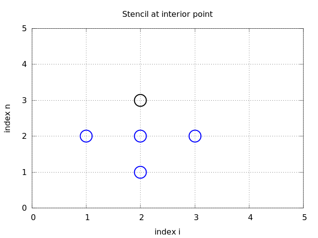
For uniformly distributed mesh points we can introduce the constant mesh spacings \( \Delta t \) and \( \Delta x \). We have that $$ \begin{equation} x_i = i\Delta x,\ i=0,\ldots,N_x,\quad t_n = n\Delta t,\ n=0,\ldots,N_t\tp \tag{2.9} \end{equation} $$ We also have that \( \Delta x = x_i-x_{i-1} \), \( i=1,\ldots,N_x \), and \( \Delta t = t_n - t_{n-1} \), \( n=1,\ldots,N_t \). Figure 24 displays a mesh in the \( x,t \) plane with \( N_t=5 \), \( N_x=5 \), and constant mesh spacings.

The discrete solution

The solution \( u(x,t) \) is sought at the mesh points. We introduce the mesh function \( u_i^n \), which approximates the exact solution at the mesh point \( (x_i,t_n) \) for \( i=0,\ldots,N_x \) and \( n=0,\ldots,N_t \). Using the finite difference method, we shall develop algebraic equations for computing the mesh function.

Fulfilling the equation at the mesh points

In the finite difference method, we relax the condition that (2.1) holds at all points in the space-time domain \( (0,L)\times (0,T] \) to the requirement that the PDE is fulfilled at the interior mesh points only: $$ \begin{equation} \frac{\partial^2}{\partial t^2} u(x_i, t_n) = c^2\frac{\partial^2}{\partial x^2} u(x_i, t_n), \tag{2.10} \end{equation} $$ for \( i=1,\ldots,N_x-1 \) and \( n=1,\ldots,N_t-1 \). For \( n=0 \) we have the initial conditions \( u=I(x) \) and \( u_t=0 \), and at the boundaries \( i=0,N_x \) we have the boundary condition \( u=0 \).

Replacing derivatives by finite differences

The second-order derivatives can be replaced by central differences. The most widely used difference approximation of the second-order derivative is $$ \frac{\partial^2}{\partial t^2}u(x_i,t_n)\approx \frac{u_i^{n+1} - 2u_i^n + u^{n-1}_i}{\Delta t^2}\tp$$ It is convenient to introduce the finite difference operator notation $$ [D_tD_t u]^n_i = \frac{u_i^{n+1} - 2u_i^n + u^{n-1}_i}{\Delta t^2}\tp$$ A similar approximation of the second-order derivative in the \( x \) direction reads $$ \frac{\partial^2}{\partial x^2}u(x_i,t_n)\approx \frac{u_{i+1}^{n} - 2u_i^n + u^{n}_{i-1}}{\Delta x^2} = [D_xD_x u]^n_i \tp $$

Algebraic version of the PDE

We can now replace the derivatives in (2.10) and get $$ \begin{equation} \frac{u_i^{n+1} - 2u_i^n + u^{n-1}_i}{\Delta t^2} = c^2\frac{u_{i+1}^{n} - 2u_i^n + u^{n}_{i-1}}{\Delta x^2}, \tag{2.11} \end{equation} $$ or written more compactly using the operator notation: $$ \begin{equation} [D_tD_t u = c^2 D_xD_x]^{n}_i \tp \tag{2.12} \end{equation} $$

Interpretation of the equation as a stencil

A characteristic feature of (2.11) is that it involves \( u \) values from neighboring points only: \( u_i^{n+1} \), \( u^n_{i\pm 1} \), \( u^n_i \), and \( u^{n-1}_i \). The circles in Figure 24 illustrate such neighboring mesh points that contribute to an algebraic equation. In this particular case, we have sampled the PDE at the point \( (2,2) \) and constructed (2.11), which then involves a coupling of \( u_nm1^1 \), \( u_n^2 \), \( u_nm1^2 \), \( u_3^2 \), and \( u_nm1^3 \). The term stencil is often used about the algebraic equation at a mesh point, and the geometry of a typical stencil is illustrated in Figure 24. One also often refers to the algebraic equations as discrete equations, (finite) difference equations or a finite difference scheme.

Algebraic version of the initial conditions

We also need to replace the derivative in the initial condition (2.3) by a finite difference approximation. A centered difference of the type $$ \frac{\partial}{\partial t} u(x_i,t_0)\approx \frac{u^1_i - u^{-1}_i}{2\Delta t} = [D_{2t} u]^0_i, $$ seems appropriate. Writing out this equation and ordering the terms give $$ \begin{equation} u^{-1}_i=u^{1}_i,\quad i=0,\ldots,N_x\tp \tag{2.13} \end{equation} $$ The other initial condition can be computed by $$ u_i^0 = I(x_i),\quad i=0,\ldots,N_x\tp$$

Formulating a recursive algorithm

We assume that \( u^n_i \) and \( u^{n-1}_i \) are available for \( i=0,\ldots,N_x \). The only unknown quantity in (2.11) is therefore \( u^{n+1}_i \), which we now can solve for: $$ \begin{equation} u^{n+1}_i = -u^{n-1}_i + 2u^n_i + C^2 \left(u^{n}_{i+1}-2u^{n}_{i} + u^{n}_{i-1}\right)\tp \tag{2.14} \end{equation} $$ We have here introduced the parameter $$ \begin{equation} C = c\frac{\Delta t}{\Delta x}, \tag{2.15} \end{equation} $$ known as the Courant number.

Given that \( u^{n-1}_i \) and \( u^n_i \) are known for \( i=0,\ldots,N_x \), we find new values at the next time level by applying the formula (2.14) for \( i=1,\ldots,N_x-1 \). Figure 24 illustrates the points that are used to compute \( u^3_2 \). For the boundary points, \( i=0 \) and \( i=N_x \), we apply the boundary conditions \( u_i^{n+1}=0 \).

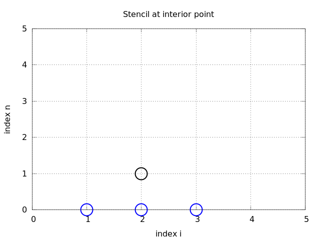
Even though sound reasoning leads up to (2.14), there is still a minor challenge with it that needs to be resolved. Think of the very first computational step to be made. The scheme (2.14) is supposed to start at \( n=1 \), which means that we compute \( u^2 \) from \( u^1 \) and \( u^0 \). Unfortunately, we do not know the value of \( u^1 \), so how to proceed? A standard procedure in such cases is to apply (2.14) also for \( n=0 \). This immediately seems strange, since it involves \( u^{-1}_i \), which is an undefined quantity outside the time mesh (and the time domain). However, we can use the initial condition (2.13) in combination with (2.14) when \( n=0 \) to eliminate \( u^{-1}_i \) and arrive at a special formula for \( u_i^1 \): $$ \begin{equation} u_i^1 = u^0_i - \half C^2\left(u^{0}_{i+1}-2u^{0}_{i} + u^{0}_{i-1}\right) \tp \tag{2.16} \end{equation} $$ Figure 25 illustrates how (2.16) connects four instead of five points: \( u^1_2 \), \( u_n^0 \), \( u_nm1^0 \), and \( u_3^0 \).

We can now summarize the computational algorithm:

1. Compute \( u^0_i=I(x_i) \) for \( i=0,\ldots,N_x \)
2. Compute \( u^1_i \) by (2.16) and set \( u_i^1=0 \) for the boundary points \( i=0 \) and \( i=N_x \), for \( n=1,2,\ldots,N-1 \),
3. For each time level \( n=1,2,\ldots,N_t-1 \)
   1. apply (2.14) to find \( u^{n+1}_i \) for \( i=1,\ldots,N_x-1 \)
   2. set \( u^{n+1}_i=0 \) for the boundary points \( i=0 \), \( i=N_x \).

Sketch of an implementation

The algorithm only involves the three most recent time levels, so we need only three arrays for \( u_i^{n+1} \), \( u_i^n \), and \( u_i^{n-1} \), \( i=0,\ldots,N_x \). Storing all the solutions in a two-dimensional array of size \( (N_x+1)\times (N_t+1) \) would be possible in this simple one-dimensional PDE problem, but is normally out of the question in three-dimensional (3D) and large two-dimensional (2D) problems. We shall therefore, in all our PDE solving programs, have the unknown in memory at as few time levels as possible.

In a Python implementation of this algorithm, we use the array elements u[i] to store \( u^{n+1}_i \), u_n[i] to store \( u^n_i \), and u_nm1[i] to store \( u^{n-1}_i \). Our naming convention is to use u for the unknown new spatial field to be computed and have all previous time levels in a list u_n that we index as u_n, u_nm1, u_n[-2] and so on. For the wave equation, u_n has just length 2.

The following Python snippet realizes the steps in the computational algorithm.

# Given mesh points as arrays x and t (x[i], t[n])
dx = x[1] - x[0]
dt = t[1] - t[0]
C = c*dt/dx            # Courant number
Nt = len(t)-1
C2 = C**2              # Help variable in the scheme

# Set initial condition u(x,0) = I(x)
for i in range(0, Nx+1):
    u_n[i] = I(x[i])

# Apply special formula for first step, incorporating du/dt=0
for i in range(1, Nx):
    u[i] = u_n[i] - \ 
           0.5*C**2(u_n[i+1] - 2*u_n[i] + u_n[i-1])
u[0] = 0;  u[Nx] = 0   # Enforce boundary conditions

# Switch variables before next step
u_nm1[:], u_n[:] = u_n, u

for n in range(1, Nt):
    # Update all inner mesh points at time t[n+1]
    for i in range(1, Nx):
        u[i] = 2u_n[i] - u_nm1[i] - \ 
               C**2(u_n[i+1] - 2*u_n[i] + u_n[i-1])

    # Insert boundary conditions
    u[0] = 0;  u[Nx] = 0

    # Switch variables before next step
    u_nm1[:], u_n[:] = u_n, u

Verification

Before implementing the algorithm, it is convenient to add a source term to the PDE (2.1), since that gives us more freedom in finding test problems for verification. Physically, a source term acts as a generator for waves in the interior of the domain.

A slightly generalized model problem

We now address the following extended initial-boundary value problem for one-dimensional wave phenomena: $$ \begin{align} u_{tt} &= c^2 u_{xx} + f(x,t), \quad &x\in (0,L),\ t\in (0,T] \tag{2.17}\\ u(x,0) &= I(x), \quad &x\in [0,L] \tag{2.18}\\ u_t(x,0) &= V(x), \quad &x\in [0,L] \tag{2.19}\\ u(0,t) & = 0, \quad &t>0 \tag{2.20}\\ u(L,t) & = 0, \quad &t>0 \tag{2.21} \end{align} $$

Sampling the PDE at \( (x_i,t_n) \) and using the same finite difference approximations as above, yields $$ \begin{equation} [D_tD_t u = c^2 D_xD_x u + f]^{n}_i \tp \tag{2.22} \end{equation} $$ Writing this out and solving for the unknown \( u^{n+1}_i \) results in $$ \begin{equation} u^{n+1}_i = -u^{n-1}_i + 2u^n_i + C^2 (u^{n}_{i+1}-2u^{n}_{i} + u^{n}_{i-1}) + \Delta t^2 f^n_i \tag{2.23} \tp \end{equation} $$

The equation for the first time step must be rederived. The discretization of the initial condition \( u_t = V(x) \) at \( t=0 \) becomes $$ [D_{2t}u = V]^0_i\quad\Rightarrow\quad u^{-1}_i = u^{1}_i - 2\Delta t V_i,$$ which, when inserted in (2.23) for \( n=0 \), gives the special formula $$ \begin{equation} u^{1}_i = u^0_i - \Delta t V_i + {\half} C^2 \left(u^{0}_{i+1}-2u^{0}_{i} + u^{0}_{i-1}\right) + \half\Delta t^2 f^0_i \tag{2.24} \tp \end{equation} $$

Using an analytical solution of physical significance

Many wave problems feature sinusoidal oscillations in time and space. For example, the original PDE problem (2.1)-(2.5) allows an exact solution $$ \begin{equation} \uex(x,t) = A\sin\left(\frac{\pi}{L}x\right) \cos\left(\frac{\pi}{L}ct\right)\tp \tag{2.25} \end{equation} $$ This \( \uex \) fulfills the PDE with \( f=0 \), boundary conditions \( \uex(0,t)=\uex(L,0)=0 \), as well as initial conditions \( I(x)=A\sin\left(\frac{\pi}{L}x\right) \) and \( V=0 \).

An introduction to the computing of convergence rates is given in the section on convergence rates in [2]. There is also a detailed example on computing convergence rates in the section Verification.

In the present problem, one expects the method to have a convergence rate of 2 (see the section Analysis of the difference equations), so if the computed rates are close to 2 on a sufficiently fine mesh, we have good evidence that the implementation is free of programming mistakes.

Manufactured solution and estimation of convergence rates

Specifying the solution and computing corresponding data

One problem with the exact solution (2.25) is that it requires a simplification (\( V=0, f=0 \)) of the implemented problem (2.17)-(2.21). An advantage of using a manufactured solution is that we can test all terms in the PDE problem. The idea of this approach is to set up some chosen solution and fit the source term, boundary conditions, and initial conditions to be compatible with the chosen solution. Given that our boundary conditions in the implementation are \( u(0,t)=u(L,t)=0 \), we must choose a solution that fulfills these conditions. One example is $$ \uex(x,t) = x(L-x)\sin t\tp$$ Inserted in the PDE \( u_{tt}=c^2u_{xx}+f \) we get $$ -x(L-x)\sin t = -c^2 2\sin t + f\quad\Rightarrow f = (2c^2 - x(L-x))\sin t\tp$$ The initial conditions become $$ \begin{align*} u(x,0) =& I(x) = 0,\\ u_t(x,0) &= V(x) = x(L-x)\tp \end{align*} $$

Defining a single discretization parameter

To verify the code, we compute the convergence rates in a series of simulations, letting each simulation use a finer mesh than the previous one. Such empirical estimation of convergence rates relies on an assumption that some measure \( E \) of the numerical error is related to the discretization parameters through $$ E = C_t\Delta t^r + C_x\Delta x^p,$$ where \( C_t \), \( C_x \), \( r \), and \( p \) are constants. The constants \( r \) and \( p \) are known as the convergence rates in time and space, respectively. From the accuracy in the finite difference approximations, we expect \( r=p=2 \), since the error terms are of order \( \Delta t^2 \) and \( \Delta x^2 \). This is confirmed by truncation error analysis and other types of analysis.

By using an exact solution of the PDE problem, we will next compute the error measure \( E \) on a sequence of refined meshes and see if the rates \( r=p=2 \) are obtained. We will not be concerned with estimating the constants \( C_t \) and \( C_x \), simply because we are not interested in their values.

It is advantageous to introduce a single discretization parameter \( h=\Delta t=\hat c \Delta x \) for some constant \( \hat c \). Since \( \Delta t \) and \( \Delta x \) are related through the Courant number, \( \Delta t = C\Delta x/c \), we set \( h=\Delta t \), and then \( \Delta x = hc/C \). Now the expression for the error measure is greatly simplified: $$ E = C_t\Delta t^r + C_x\Delta x^r = C_t h^r + C_x\left(\frac{c}{C}\right)^r h^r = Dh^r,\quad D = C_t+C_x\left(\frac{c}{C}\right)^r \tp$$

Computing errors

We choose an initial discretization parameter \( h_0 \) and run experiments with decreasing \( h \): \( h_i=2^{-i}h_0 \), \( i=1,2,\ldots,m \). Halving \( h \) in each experiment is not necessary, but it is a common choice. For each experiment we must record \( E \) and \( h \). A standard choice of error measure is the \( \ell^2 \) or \( \ell^\infty \) norm of the error mesh function \( e^n_i \): $$ \begin{align} E &= ||e^n_i||_{\ell^2} = \left( \Delta t\Delta x \sum_{n=0}^{N_t}\sum_{i=0}^{N_x} (e^n_i)^2\right)^{\half},\quad e^n_i = \uex(x_i,t_n)-u^n_i, \tag{2.26}\\ E &= ||e^n_i||_{\ell^\infty} = \max_{i,n} |e^i_n|\tp \tag{2.27} \end{align} $$ In Python, one can compute \( \sum_{i}(e^{n}_i)^2 \) at each time step and accumulate the value in some sum variable, say e2_sum. At the final time step one can do sqrt(dt*dx*e2_sum). For the \( \ell^\infty \) norm one must compare the maximum error at a time level (e.max()) with the global maximum over the time domain: e_max = max(e_max, e.max()).

An alternative error measure is to use a spatial norm at one time step only, e.g., the end time \( T \) (\( n=N_t \)): $$ \begin{align} E &= ||e^n_i||_{\ell^2} = \left( \Delta x\sum_{i=0}^{N_x} (e^n_i)^2\right)^{\half},\quad e^n_i = \uex(x_i,t_n)-u^n_i, \tag{2.28}\\ E &= ||e^n_i||_{\ell^\infty} = \max_{0\leq i\leq N_x} |e^{n}_i|\tp \tag{2.29} \end{align} $$ The important issue is that our error measure \( E \) must be one number that represents the error in the simulation.

Computing rates

Let \( E_i \) be the error measure in experiment (mesh) number \( i \) and let \( h_i \) be the corresponding discretization parameter (\( h \)). With the error model \( E_i = Dh_i^r \), we can estimate \( r \) by comparing two consecutive experiments: $$ \begin{align*} E_{i+1}& =D h_{i+1}^{r},\\ E_{i}& =D h_{i}^{r}\tp \end{align*} $$ Dividing the two equations eliminates the (uninteresting) constant \( D \). Thereafter, solving for \( r \) yields $$ r = \frac{\ln E_{i+1}/E_{i}}{\ln h_{i+1}/h_{i}}\tp $$ Since \( r \) depends on \( i \), i.e., which simulations we compare, we add an index to \( r \): \( r_i \), where \( i=0,\ldots,m-2 \), if we have \( m \) experiments: \( (h_0,E_0),\ldots,(h_{m-1}, E_{m-1}) \).

In our present discretization of the wave equation we expect \( r=2 \), and hence the \( r_i \) values should converge to 2 as \( i \) increases.

Constructing an exact solution of the discrete equations

With a manufactured or known analytical solution, as outlined above, we can estimate convergence rates and see if they have the correct asymptotic behavior. Experience shows that this is a quite good verification technique in that many common bugs will destroy the convergence rates. A significantly better test though, would be to check that the numerical solution is exactly what it should be. This will in general require exact knowledge of the numerical error, which we do not normally have (although we in the section Analysis of the difference equations establish such knowledge in simple cases). However, it is possible to look for solutions where we can show that the numerical error vanishes, i.e., the solution of the original continuous PDE problem is also a solution of the discrete equations. This property often arises if the exact solution of the PDE is a lower-order polynomial. (Truncation error analysis leads to error measures that involve derivatives of the exact solution. In the present problem, the truncation error involves 4th-order derivatives of \( u \) in space and time. Choosing \( u \) as a polynomial of degree three or less will therefore lead to vanishing error.)

We shall now illustrate the construction of an exact solution to both the PDE itself and the discrete equations. Our chosen manufactured solution is quadratic in space and linear in time. More specifically, we set $$ \begin{equation} \uex (x,t) = x(L-x)(1+{\half}t), \tag{2.30} \end{equation} $$ which by insertion in the PDE leads to \( f(x,t)=2(1+t)c^2 \). This \( \uex \) fulfills the boundary conditions \( u=0 \) and demands \( I(x)=x(L-x) \) and \( V(x)={\half}x(L-x) \).

To realize that the chosen \( \uex \) is also an exact solution of the discrete equations, we first remind ourselves that \( t_n=n\Delta t \) before we establish that $$ \begin{align} \lbrack D_tD_t t^2\rbrack^n &= \frac{t_{n+1}^2 - 2t_n^2 + t_{n-1}^2}{\Delta t^2} = (n+1)^2 -2n^2 + (n-1)^2 = 2, \tag{2.31}\\ \lbrack D_tD_t t\rbrack^n &= \frac{t_{n+1} - 2t_n + t_{n-1}}{\Delta t^2} = \frac{((n+1) -2n + (n-1))\Delta t}{\Delta t^2} = 0 \tp \tag{2.32} \end{align} $$ Hence, $$ [D_tD_t \uex]^n_i = x_i(L-x_i)[D_tD_t (1+{\half}t)]^n = x_i(L-x_i){\half}[D_tD_t t]^n = 0\tp$$ Similarly, we get that $$ \begin{align*} \lbrack D_xD_x \uex\rbrack^n_i &= (1+{\half}t_n)\lbrack D_xD_x (xL-x^2)\rbrack_i\\ & = (1+{\half}t_n)\lbrack LD_xD_x x - D_xD_x x^2\rbrack_i \\ &= -2(1+{\half}t_n) \tp \end{align*} $$ Now, \( f^n_i = 2(1+{\half}t_n)c^2 \), which results in $$ [D_tD_t \uex - c^2D_xD_x\uex - f]^n_i = 0 + c^2 2(1 + {\half}t_{n}) + 2(1+{\half}t_n)c^2 = 0\tp$$

Moreover, \( \uex(x_i,0)=I(x_i) \), \( \partial \uex/\partial t = V(x_i) \) at \( t=0 \), and \( \uex(x_0,t)=\uex(x_{N_x},0)=0 \). Also the modified scheme for the first time step is fulfilled by \( \uex(x_i,t_n) \).

Therefore, the exact solution \( \uex(x,t)=x(L-x)(1+t/2) \) of the PDE problem is also an exact solution of the discrete problem. This means that we know beforehand what numbers the numerical algorithm should produce. We can use this fact to check that the computed \( u^n_i \) values from an implementation equals \( \uex(x_i,t_n) \), within machine precision. This result is valid regardless of the mesh spacings \( \Delta x \) and \( \Delta t \)! Nevertheless, there might be stability restrictions on \( \Delta x \) and \( \Delta t \), so the test can only be run for a mesh that is compatible with the stability criterion (which in the present case is \( C\leq 1 \), to be derived later).

Implementation

This section presents the complete computational algorithm, its implementation in Python code, animation of the solution, and verification of the implementation.

A real implementation of the basic computational algorithm from the sections Formulating a recursive algorithm and Sketch of an implementation can be encapsulated in a function, taking all the input data for the problem as arguments. The physical input data consists of \( c \), \( I(x) \), \( V(x) \), \( f(x,t) \), \( L \), and \( T \). The numerical input is the mesh parameters \( \Delta t \) and \( \Delta x \).

Instead of specifying \( \Delta t \) and \( \Delta x \), we can specify one of them and the Courant number \( C \) instead, since having explicit control of the Courant number is convenient when investigating the numerical method. Many find it natural to prescribe the resolution of the spatial grid and set \( N_x \). The solver function can then compute \( \Delta t = CL/(cN_x) \). However, for comparing \( u(x,t) \) curves (as functions of \( x \)) for various Courant numbers it is more convenient to keep \( \Delta t \) fixed for all \( C \) and let \( \Delta x \) vary according to \( \Delta x = c\Delta t/C \). With \( \Delta t \) fixed, all frames correspond to the same time \( t \), and this simplifies animations that compare simulations with different mesh resolutions. Plotting functions of \( x \) with different spatial resolution is trivial, so it is easier to let \( \Delta x \) vary in the simulations than \( \Delta t \).

Callback function for user-specific actions

The solution at all spatial points at a new time level is stored in an array u of length \( N_x+1 \). We need to decide what to do with this solution, e.g., visualize the curve, analyze the values, or write the array to file for later use. The decision about what to do is left to the user in the form of a user-supplied function

user_action(u, x, t, n)

where u is the solution at the spatial points x at time t[n]. The user_action function is called from the solver at each time level n.

If the user wants to plot the solution or store the solution at a time point, she needs to write such a function and take appropriate actions inside it. We will show examples on many such user_action functions.

Since the solver function makes calls back to the user's code via such a function, this type of function is called a callback function. When writing general software, like our solver function, which also needs to carry out special problem- or solution-dependent actions (like visualization), it is a common technique to leave those actions to user-supplied callback functions.

The callback function can be used to terminate the solution process if the user returns True. For example,

def my_user_action_function(u, x, t, n):
    return np.abs(u).max() > 10

is a callback function that will terminate the solver function of the amplitude of the waves exceed 10, which is here considered as a numerical instability.

The solver function

A first attempt at a solver function is listed below.

import numpy as np

def solver(I, V, f, c, L, dt, C, T, user_action=None):
    """Solve u_tt=c^2*u_xx + f on (0,L)x(0,T]."""
    Nt = int(round(T/dt))
    t = np.linspace(0, Nt*dt, Nt+1)   # Mesh points in time
    dx = dt*c/float(C)
    Nx = int(round(L/dx))
    x = np.linspace(0, L, Nx+1)       # Mesh points in space
    C2 = C**2                         # Help variable in the scheme
    # Make sure dx and dt are compatible with x and t
    dx = x[1] - x[0]
    dt = t[1] - t[0]

    if f is None or f == 0 :
        f = lambda x, t: 0
    if V is None or V == 0:
        V = lambda x: 0

    u     = np.zeros(Nx+1)   # Solution array at new time level
    u_n   = np.zeros(Nx+1)   # Solution at 1 time level back
    u_nm1 = np.zeros(Nx+1)   # Solution at 2 time levels back

    import time;  t0 = time.clock()  # Measure CPU time

    # Load initial condition into u_n
    for i in range(0,Nx+1):
        u_n[i] = I(x[i])

    if user_action is not None:
        user_action(u_n, x, t, 0)

    # Special formula for first time step
    n = 0
    for i in range(1, Nx):
        u[i] = u_n[i] + dt*V(x[i]) + \ 
               0.5*C2*(u_n[i-1] - 2*u_n[i] + u_n[i+1]) + \ 
               0.5*dt**2*f(x[i], t[n])
    u[0] = 0;  u[Nx] = 0

    if user_action is not None:
        user_action(u, x, t, 1)

    # Switch variables before next step
    u_nm1[:] = u_n;  u_n[:] = u

    for n in range(1, Nt):
        # Update all inner points at time t[n+1]
        for i in range(1, Nx):
            u[i] = - u_nm1[i] + 2*u_n[i] + \ 
                     C2*(u_n[i-1] - 2*u_n[i] + u_n[i+1]) + \ 
                     dt**2*f(x[i], t[n])

        # Insert boundary conditions
        u[0] = 0;  u[Nx] = 0
        if user_action is not None:
            if user_action(u, x, t, n+1):
                break

        # Switch variables before next step
        u_nm1[:] = u_n;  u_n[:] = u

    cpu_time = time.clock() - t0
    return u, x, t, cpu_time

A couple of remarks about the above code is perhaps necessary:

• Although we give dt and compute dx via C and c, the resulting t and x meshes do not necessarily correspond exactly to these values because of rounding errors. To explicitly ensure that dx and dt correspond to the cell sizes in x and t, we recompute the values.
• According to the convention described in the section Callback function for user-specific actions, a true value returned from user_action should terminate the simulation, here implemented by a break statement inside the for loop in the solver.

Verification: exact quadratic solution

We use the test problem derived in the section A slightly generalized model problem for verification. Below is a unit test based on this test problem and realized as a proper test function compatible with the unit test frameworks nose or pytest.

def test_quadratic():
    """Check that u(x,t)=x(L-x)(1+t/2) is exactly reproduced."""

    def u_exact(x, t):
        return x*(L-x)*(1 + 0.5*t)

    def I(x):
        return u_exact(x, 0)

    def V(x):
        return 0.5*u_exact(x, 0)

    def f(x, t):
        return 2*(1 + 0.5*t)*c**2

    L = 2.5
    c = 1.5
    C = 0.75
    Nx = 6  # Very coarse mesh for this exact test
    dt = C*(L/Nx)/c
    T = 18

    def assert_no_error(u, x, t, n):
        u_e = u_exact(x, t[n])
        diff = np.abs(u - u_e).max()
        tol = 1E-13
        assert diff < tol

    solver(I, V, f, c, L, dt, C, T,
           user_action=assert_no_error)

When this function resides in the file wave1D_u0.py, one can run pytest to check that all test functions with names test_*() in this file work:

Terminal> py.test -s -v wave1D_u0.py

Verification: convergence rates

A more general method, but not so reliable as a verification method, is to compute the convergence rates and see if they coincide with theoretical estimates. Here we expect a rate of 2 according to the various results in the section Analysis of the difference equations. A general function for computing convergence rates can be written like this:

def convergence_rates(
    u_exact,                 # Python function for exact solution
    I, V, f, c, L,           # physical parameters
    dt0, num_meshes, C, T):  # numerical parameters
    """
    Half the time step and estimate convergence rates for
    for num_meshes simulations.
    """
    # First define an appropriate user action function
    global error
    error = 0  # error computed in the user action function

    def compute_error(u, x, t, n):
        global error  # must be global to be altered here
        # (otherwise error is a local variable, different
        # from error defined in the parent function)
        if n == 0:
            error = 0
        else:
            error = max(error, np.abs(u - u_exact(x, t[n])).max())

    # Run finer and finer resolutions and compute true errors
    E = []
    h = []  # dt, solver adjusts dx such that C=dt*c/dx
    dt = dt0
    for i in range(num_meshes):
        solver(I, V, f, c, L, dt, C, T,
               user_action=compute_error)
        # error is computed in the final call to compute_error
        E.append(error)
        h.append(dt)
        dt /= 2  # halve the time step for next simulation
    print 'E:', E
    print 'h:', h
    # Convergence rates for two consecutive experiments
    r = [np.log(E[i]/E[i-1])/np.log(h[i]/h[i-1])
         for i in range(1,num_meshes)]
    return r

Using the analytical solution from the section Using an analytical solution of physical significance, we can call convergece_rates to see if we get a convergence rate that approaches 2 and use the final estimate of the rate in an assert statement such that this function becomes a proper test function:

def test_convrate_sincos():
    n = m = 2
    L = 1.0
    u_exact = lambda x, t: np.cos(m*np.pi/L*t)*np.sin(m*np.pi/L*x)

    r = convergence_rates(
        u_exact=u_exact,
        I=lambda x: u_exact(x, 0),
        V=lambda x: 0,
        f=0,
        c=1,
        L=L,
        dt0=0.1,
        num_meshes=6,
        C=0.9,
        T=1)
    print 'rates sin(x)*cos(t) solution:', \ 
          [round(r_,2) for r_ in r]
    assert abs(r[-1] - 2) < 0.002

Doing py.test -s -v wave1D_u0.py will run also this test function and show the rates 2.05, 1.98, 2.0, 2.0, and 2.0 (to two decimals).

Visualization: animating the solution

Now that we have verified the implementation it is time to do a real computation where we also display evolution of the waves on the screen. Since the solver function knows nothing about what type of visualizations we may want, it calls the callback function user_action(u, x, t, n). We must therefore write this function and find the proper statements for plotting the solution.

Function for administering the simulation

The following viz function

1. defines a user_action callback function for plotting the solution at each time level,
2. calls the solver function, and
3. combines all the plots (in files) to video in different formats.

def viz(
    I, V, f, c, L, dt, C, T,  # PDE parameters
    umin, umax,               # Interval for u in plots
    animate=True,             # Simulation with animation?
    tool='matplotlib',        # 'matplotlib' or 'scitools'
    solver_function=solver,   # Function with numerical algorithm
    ):
    """Run solver and visualize u at each time level."""

    def plot_u_st(u, x, t, n):
        """user_action function for solver."""
        plt.plot(x, u, 'r-',
                 xlabel='x', ylabel='u',
                 axis=[0, L, umin, umax],
                 title='t=%f' % t[n], show=True)
        # Let the initial condition stay on the screen for 2
        # seconds, else insert a pause of 0.2 s between each plot
        time.sleep(2) if t[n] == 0 else time.sleep(0.2)
        plt.savefig('frame_%04d.png' % n)  # for movie making

    class PlotMatplotlib:
        def __call__(self, u, x, t, n):
            """user_action function for solver."""
            if n == 0:
                plt.ion()
                self.lines = plt.plot(x, u, 'r-')
                plt.xlabel('x');  plt.ylabel('u')
                plt.axis([0, L, umin, umax])
                plt.legend(['t=%f' % t[n]], loc='lower left')
            else:
                self.lines[0].set_ydata(u)
                plt.legend(['t=%f' % t[n]], loc='lower left')
                plt.draw()
            time.sleep(2) if t[n] == 0 else time.sleep(0.2)
            plt.savefig('tmp_%04d.png' % n)  # for movie making

    if tool == 'matplotlib':
        import matplotlib.pyplot as plt
        plot_u = PlotMatplotlib()
    elif tool == 'scitools':
        import scitools.std as plt  # scitools.easyviz interface
        plot_u = plot_u_st
    import time, glob, os

    # Clean up old movie frames
    for filename in glob.glob('tmp_*.png'):
        os.remove(filename)

    # Call solver and do the simulaton
    user_action = plot_u if animate else None
    u, x, t, cpu = solver_function(
        I, V, f, c, L, dt, C, T, user_action)

    # Make video files
    fps = 4  # frames per second
    codec2ext = dict(flv='flv', libx264='mp4', libvpx='webm',
                     libtheora='ogg')  # video formats
    filespec = 'tmp_%04d.png'
    movie_program = 'ffmpeg'  # or 'avconv'
    for codec in codec2ext:
        ext = codec2ext[codec]
        cmd = '%(movie_program)s -r %(fps)d -i %(filespec)s '\ 
              '-vcodec %(codec)s movie.%(ext)s' % vars()
        os.system(cmd)

    if tool == 'scitools':
        # Make an HTML play for showing the animation in a browser
        plt.movie('tmp_*.png', encoder='html', fps=fps,
                  output_file='movie.html')
    return cpu

Dissection of the code

The viz function can either use SciTools or Matplotlib for visualizing the solution. The user_action function based on SciTools is called plot_u_st, while the user_action function based on Matplotlib is a bit more complicated as it is realized as a class and needs statements that differ from those for making static plots. SciTools can utilize both Matplotlib and Gnuplot (and many other plotting programs) for doing the graphics, but Gnuplot is a relevant choice for large \( N_x \) or in two-dimensional problems as Gnuplot is significantly faster than Matplotlib for screen animations.

A function inside another function, like plot_u_st in the above code segment, has access to and remembers all the local variables in the surrounding code inside the viz function (!). This is known in computer science as a closure and is very convenient to program with. For example, the plt and time modules defined outside plot_u are accessible for plot_u_st when the function is called (as user_action) in the solver function. Some may think, however, that a class instead of a closure is a cleaner and easier-to-understand implementation of the user action function, see the section Building a general 1D wave equation solver.

The plot_u_st function just makes a standard SciTools plot command for plotting u as a function of x at time t[n]. To achieve a smooth animation, the plot command should take keyword arguments instead of being broken into separate calls to xlabel, ylabel, axis, time, and show. Several plot calls will automatically cause an animation on the screen. In addition, we want to save each frame in the animation to file. We then need a filename where the frame number is padded with zeros, here tmp_0000.png, tmp_0001.png, and so on. The proper printf construction is then tmp_%04d.png. The section Making animations contains more basic information on making animations.

The solver is called with an argument plot_u as user_function. If the user chooses to use SciTools, plot_u is the plot_u_st callback function, but for Matplotlib it is an instance of the class PlotMatplotlib. Also this class makes use of variables defined in the viz function: plt and time. With Matplotlib, one has to make the first plot the standard way, and then update the \( y \) data in the plot at every time level. The update requires active use of the returned value from plt.plot in the first plot. This value would need to be stored in a local variable if we were to use a closure for the user_action function when doing the animation with Matplotlib. It is much easier to store the variable as a class attribute self.lines. Since the class is essentially a function, we implement the function as the special method __call__ such that the instance plot_u(u, x, t, n) can be called as a standard callback function from solver.

Making movie files

From the frame_*.png files containing the frames in the animation we can make video files. The section Making animations presents basic information on how to use the ffmpeg (or avconv) program for producing video files in different modern formats: Flash, MP4, Webm, and Ogg.

The viz function creates an ffmpeg or avconv command with the proper arguments for each of the formats Flash, MP4, WebM, and Ogg. The task is greatly simplified by having a codec2ext dictionary for mapping video codec names to filename extensions. As mentioned in the section Making animations, only two formats are actually needed to ensure that all browsers can successfully play the video: MP4 and WebM.

Some animations having a large number of plot files may not be properly combined into a video using ffmpeg or avconv. A method that always works is to play the PNG files as an animation in a browser using JavaScript code in an HTML file. The SciTools package has a function movie (or a stand-alone command scitools movie) for creating such an HTML player. The plt.movie call in the viz function shows how the function is used. The file movie.html can be loaded into a browser and features a user interface where the speed of the animation can be controlled. Note that the movie in this case consists of the movie.html file and all the frame files tmp_*.png.

Skipping frames for animation speed

Sometimes the time step is small and \( T \) is large, leading to an inconveniently large number of plot files and a slow animation on the screen. The solution to such a problem is to decide on a total number of frames in the animation, num_frames, and plot the solution only for every skip_frame frames. For example, setting skip_frame=5 leads to plots of every 5 frames. The default value skip_frame=1 plots every frame. The total number of time levels (i.e., maximum possible number of frames) is the length of t, t.size (or len(t)), so if we want num_frames frames in the animation, we need to plot every t.size/num_frames frames:

skip_frame = int(t.size/float(num_frames))
if n % skip_frame == 0 or n == t.size-1:
    st.plot(x, u, 'r-', ...)

The initial condition (n=0) is included by n % skip_frame == 0, as well as every skip_frame-th frame. As n % skip_frame == 0 will very seldom be true for the very final frame, we must also check if n == t.size-1 to get the final frame included.

A simple choice of numbers may illustrate the formulas: say we have 801 frames in total (t.size) and we allow only 60 frames to be plotted. As n then runs from 801 to 0, we need to plot every 801/60 frame, which with integer division yields 13 as skip_frame. Using the mod function, n % skip_frame, this operation is zero every time n can be divided by 13 without a remainder. That is, the if test is true when n equals \( 0, 13, 26, 39, ..., 780, 801 \). The associated code is included in the plot_u function, inside the viz function, in the file wave1D_u0.py.

Running a case

The first demo of our 1D wave equation solver concerns vibrations of a string that is initially deformed to a triangular shape, like when picking a guitar string: $$ \begin{equation} I(x) = \left\lbrace \begin{array}{ll} ax/x_0, & x < x_0,\\ a(L-x)/(L-x_0), & \hbox{otherwise} \end{array}\right. \tag{2.33} \end{equation} $$ We choose \( L=75 \) cm, \( x_0=0.8L \), \( a=5 \) mm, and a time frequency \( \nu = 440 \) Hz. The relation between the wave speed \( c \) and \( \nu \) is \( c=\nu\lambda \), where \( \lambda \) is the wavelength, taken as \( 2L \) because the longest wave on the string forms half a wavelength. There is no external force, so \( f=0 \) (meaning we can neglect gravity), and the string is at rest initially, implying \( V=0 \).

Regarding numerical parameters, we need to specify a \( \Delta t \). Sometimes it is more natural to think of a spatial resolution instead of a time step. A natural semi-coarse spatial resolution in the present problem is \( N_x=50 \). We can then choose the associated \( \Delta t \) (as required by the viz and solver functions) as the stability limit: \( \Delta t = L/(N_xc) \). This is the \( \Delta t \) to be specified, but notice that if \( C < 1 \), the actual \( \Delta x \) computed in solver gets larger than \( L/N_x \): \( \Delta x = c\Delta t/C = L/(N_xC) \). (The reason is that we fix \( \Delta t \) and adjust \( \Delta x \), so if \( C \) gets smaller, the code implements this effect in terms of a larger \( \Delta x \).)

A function for setting the physical and numerical parameters and calling viz in this application goes as follows:

def guitar(C):
    """Triangular wave (pulled guitar string)."""
    L = 0.75
    x0 = 0.8*L
    a = 0.005
    freq = 440
    wavelength = 2*L
    c = freq*wavelength
    omega = 2*pi*freq
    num_periods = 1
    T = 2*pi/omega*num_periods
    # Choose dt the same as the stability limit for Nx=50
    dt = L/50./c

    def I(x):
        return a*x/x0 if x < x0 else a/(L-x0)*(L-x)

    umin = -1.2*a;  umax = -umin
    cpu = viz(I, 0, 0, c, L, dt, C, T, umin, umax,
              animate=True, tool='scitools')

The associated program has the name wave1D_u0.py. Run the program and watch the movie of the vibrating string. The string should ideally consist of straight segments, but these are somewhat wavy due to numerical approximation. Run the case with the wave1D_u0.py code and \( C=1 \) to see the exact solution.

Working with a scaled PDE model

Depending on the model, it may be a substantial job to establish consistent and relevant physical parameter values for a case. The guitar string example illustrates the point. However, by scaling the mathematical problem we can often reduce the need to estimate physical parameters dramatically. The scaling technique consists of introducing new independent and dependent variables, with the aim that the absolute values of these lie in \( [0,1] \). We introduce the dimensionless variables (details are found in the section Homogeneous Dirichlet conditions in 1D in the book Scaling of differential equations [3] $$ \bar x = \frac{x}{L},\quad \bar t = \frac{c}{L}t,\quad \bar u = \frac{u}{a} \tp $$ Here, \( L \) is a typical length scale, e.g., the length of the domain, and \( a \) is a typical size of \( u \), e.g., determined from the initial condition: \( a=\max_x|I(x)| \).

We get by the chain rule that $$ \frac{\partial u}{\partial t} = \frac{\partial}{\partial\bar t}\left(a\bar u\right) \frac{d\bar t}{dt} = \frac{ac}{L}\frac{\partial\bar u}{\partial\bar t}\tp$$ Similarly, $$ \frac{\partial u}{\partial x} = \frac{a}{L}\frac{\partial\bar u}{\partial\bar x}\tp$$ Inserting the dimensionless variables in the PDE gives, in case \( f=0 \), $$ \frac{a^2c^2}{L^2}\frac{\partial^2\bar u}{\partial\bar t^2} = \frac{a^2c^2}{L^2}\frac{\partial^2\bar u}{\partial\bar x^2}\tp$$ Dropping the bars, we arrive at the scaled PDE $$ \begin{equation} \frac{\partial^2 u}{\partial t^2} = \frac{\partial^2 u}{\partial x^2}, \quad x\in (0,1),\ t\in (0,cT/L), \tag{2.34} \end{equation} $$ which has no parameter \( c^2 \) anymore. The initial conditions are scaled as $$ a\bar u(\bar x, 0) = I(L\bar x)$$ and $$ \frac{a}{L/c}\frac{\partial\bar u}{\partial\bar t}(\bar x,0) = V(L\bar x),$$ resulting in $$ \bar u(\bar x, 0) = \frac{I(L\bar x)}{\max_x |I(x)|},\quad \frac{\partial\bar u}{\partial\bar t}(\bar x,0) = \frac{L}{ac}V(L\bar x)\tp$$ In the common case \( V=0 \) we see that there are no physical parameters to be estimated in the PDE model!

If we have a program implemented for the physical wave equation with dimensions, we can obtain the dimensionless, scaled version by setting \( c=1 \). The initial condition of a guitar string, given in (2.33), gets its scaled form by choosing \( a=1 \), \( L=1 \), and \( x_0\in [0,1] \). This means that we only need to decide on the \( x_0 \) value as a fraction of unity, because the scaled problem corresponds to setting all other parameters to unity. In the code we can just set a=c=L=1, x0=0.8, and there is no need to calculate with wavelengths and frequencies to estimate \( c \)!

The only non-trivial parameter to estimate in the scaled problem is the final end time of the simulation, or more precisely, how it relates to periods in periodic solutions in time, since we often want to express the end time as a certain number of periods. The period in the dimensionless problem is 2, so the end time can be set to the desired number of periods times 2.

Why the dimensionless period is 2 can be explained by the following reasoning. Suppose that \( u \) behaves as \( \cos (\omega t) \) in time in the original problem with dimensions. The corresponding period is then \( P=2\pi/\omega \), but we need to estimate \( \omega \). A typical solution of the wave equation is \( u(x,t)=A\cos(kx)\cos(\omega t) \), where \( A \) is an amplitude and \( k \) is related to the wave length \( \lambda \) in space: \( \lambda = 2\pi/k \). Both \( \lambda \) and \( A \) will be given by the initial condition \( I(x) \). Inserting this \( u(x,t) \) in the PDE yields \( -\omega^2 = -c^2k^2 \), i.e., \( \omega = kc \). The period is therefore \( P=2\pi/(kc) \). If the boundary conditions are \( u(0,t)=u(L,t) \), we need to have \( kL = n\pi \) for integer \( n \). The period becomes \( P=2L/nc \). The longest period is \( P=2L/c \). The dimensionless period \( \tilde P \) is obtained by dividing \( P \) by the time scale \( L/c \), which results in \( \tilde P=2 \). Shorter waves in the initial condition will have a dimensionless shorter period \( \tilde P=2/n \) (\( n>1 \)).

Vectorization

The computational algorithm for solving the wave equation visits one mesh point at a time and evaluates a formula for the new value \( u_i^{n+1} \) at that point. Technically, this is implemented by a loop over array elements in a program. Such loops may run slowly in Python (and similar interpreted languages such as R and MATLAB). One technique for speeding up loops is to perform operations on entire arrays instead of working with one element at a time. This is referred to as vectorization, vector computing, or array computing. Operations on whole arrays are possible if the computations involving each element is independent of each other and therefore can, at least in principle, be performed simultaneously. That is, vectorization not only speeds up the code on serial computers, but also makes it easy to exploit parallel computing. Actually, there are Python tools like Numba that can automatically turn vectorized code into parallel code.

Operations on slices of arrays

Efficient computing with numpy arrays demands that we avoid loops and compute with entire arrays at once (or at least large portions of them). Consider this calculation of differences \( d_i = u_{i+1}-u_i \):

n = u.size
for i in range(0, n-1):
    d[i] = u[i+1] - u[i]

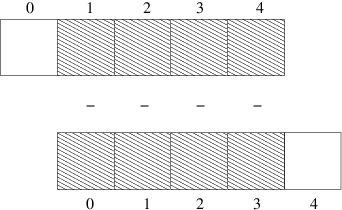
All the differences here are independent of each other. The computation of d can therefore alternatively be done by subtracting the array \( (u_0,u_n,\ldots,u_{n-1}) \) from the array where the elements are shifted one index upwards: \( (u_n,u_nm1,\ldots,u_n) \), see Figure 26. The former subset of the array can be expressed by u[0:n-1], u[0:-1], or just u[:-1], meaning from index 0 up to, but not including, the last element (-1). The latter subset is obtained by u[1:n] or u[1:], meaning from index 1 and the rest of the array. The computation of d can now be done without an explicit Python loop:

d = u[1:] - u[:-1]

or with explicit limits if desired:

d = u[1:n] - u[0:n-1]

Indices with a colon, going from an index to (but not including) another index are called slices. With numpy arrays, the computations are still done by loops, but in efficient, compiled, highly optimized C or Fortran code. Such loops are sometimes referred to as vectorized loops. Such loops can also easily be distributed among many processors on parallel computers. We say that the scalar code above, working on an element (a scalar) at a time, has been replaced by an equivalent vectorized code. The process of vectorizing code is called vectorization.

Finite difference schemes basically contain differences between array elements with shifted indices. As an example, consider the updating formula

for i in range(1, n-1):
    u2[i] = u[i-1] - 2*u[i] + u[i+1]

The vectorization consists of replacing the loop by arithmetics on slices of arrays of length n-2:

u2 = u[:-2] - 2*u[1:-1] + u[2:]
u2 = u[0:n-2] - 2*u[1:n-1] + u[2:n]   # alternative

Note that the length of u2 becomes n-2. If u2 is already an array of length n and we want to use the formula to update all the "inner" elements of u2, as we will when solving a 1D wave equation, we can write

u2[1:-1]  = u[:-2] - 2*u[1:-1] + u[2:]
u2[1:n-1] = u[0:n-2] - 2*u[1:n-1] + u[2:n]   # alternative

The first expression's right-hand side is realized by the following steps, involving temporary arrays with intermediate results, since each array operation can only involve one or two arrays. The numpy package performs (behind the scenes) the first line above in four steps:

temp1 = 2*u[1:-1]
temp2 = u[:-2] - temp1
temp3 = temp2 + u[2:]
u2[1:-1] = temp3

We need three temporary arrays, but a user does not need to worry about such temporary arrays.

u2[1:n-1] = u[0:n-2] - 2*u[1:n-1] + u[2:n]

u2[1:n-1] = u[0:n-2] - 2*u[1:n-1] + u[1:n]

u2 = u[0:n-2] - 2*u[1:n-1] + u[1:n]

Vectorization may also work nicely with functions. To illustrate, we may extend the previous example as follows:

def f(x):
    return x**2 + 1

for i in range(1, n-1):
    u2[i] = u[i-1] - 2*u[i] + u[i+1] + f(x[i])

Assuming u2, u, and x all have length n, the vectorized version becomes

u2[1:-1] = u[:-2] - 2*u[1:-1] + u[2:] + f(x[1:-1])

Obviously, f must be able to take an array as argument for f(x[1:-1]) to make sense.

Finite difference schemes expressed as slices

We now have the necessary tools to vectorize the wave equation algorithm as described mathematically in the section Formulating a recursive algorithm and through code in the section The solver function. There are three loops: one for the initial condition, one for the first time step, and finally the loop that is repeated for all subsequent time levels. Since only the latter is repeated a potentially large number of times, we limit our vectorization efforts to this loop:

for i in range(1, Nx):
    u[i] = 2*u_n[i] - u_nm1[i] + \ 
           C2*(u_n[i-1] - 2*u_n[i] + u_n[i+1])

The vectorized version becomes

u[1:-1] = - u_nm1[1:-1] + 2*u_n[1:-1] + \ 
          C2*(u_n[:-2] - 2*u_n[1:-1] + u_n[2:])

or

u[1:Nx] = 2*u_n[1:Nx]- u_nm1[1:Nx] + \ 
          C2*(u_n[0:Nx-1] - 2*u_n[1:Nx] + u_n[2:Nx+1])

The program wave1D_u0v.py contains a new version of the function solver where both the scalar and the vectorized loops are included (the argument version is set to scalar or vectorized, respectively).

Verification

We may reuse the quadratic solution \( \uex(x,t)=x(L-x)(1+{\half}t) \) for verifying also the vectorized code. A test function can now verify both the scalar and the vectorized version. Moreover, we may use a user_action function that compares the computed and exact solution at each time level and performs a test:

def test_quadratic():
    """
    Check the scalar and vectorized versions for
    a quadratic u(x,t)=x(L-x)(1+t/2) that is exactly reproduced.
    """
    # The following function must work for x as array or scalar
    u_exact = lambda x, t: x*(L - x)*(1 + 0.5*t)
    I = lambda x: u_exact(x, 0)
    V = lambda x: 0.5*u_exact(x, 0)
    # f is a scalar (zeros_like(x) works for scalar x too)
    f = lambda x, t: np.zeros_like(x) + 2*c**2*(1 + 0.5*t)

    L = 2.5
    c = 1.5
    C = 0.75
    Nx = 3  # Very coarse mesh for this exact test
    dt = C*(L/Nx)/c
    T = 18

    def assert_no_error(u, x, t, n):
        u_e = u_exact(x, t[n])
        tol = 1E-13
        diff = np.abs(u - u_e).max()
        assert diff < tol

    solver(I, V, f, c, L, dt, C, T,
           user_action=assert_no_error, version='scalar')
    solver(I, V, f, c, L, dt, C, T,
           user_action=assert_no_error, version='vectorized')

f = lambda x, t: L*(x-t)**2

def f(x, t):
    return L(x-t)**2

solver(I=lambda x: sin(pi*x/L), V=0, f=0, ...)

Efficiency measurements

The wave1D_u0v.py contains our new solver function with both scalar and vectorized code. For comparing the efficiency of scalar versus vectorized code, we need a viz function as discussed in the section Visualization: animating the solution. All of this viz function can be reused, except the call to solver_function. This call lacks the parameter version, which we want to set to vectorized and scalar for our efficiency measurements.

One solution is to copy the viz code from wave1D_u0 into wave1D_u0v.py and add a version argument to the solver_function call. Taking into account how much animation code we then duplicate, this is not a good idea. Alternatively, introducing the version argument in wave1D_u0.viz, so that this function can be imported into wave1D_u0v.py, is not a good solution either, since version has no meaning in that file. We need better ideas!

Solution 1

Calling viz in wave1D_u0 with solver_function as our new solver in wave1D_u0v works fine, since this solver has version='vectorized' as default value. The problem arises when we want to test version='scalar'. The simplest solution is then to use wave1D_u0.solver instead. We make a new viz function in wave1D_u0v.py that has a version argument and that just calls wave1D_u0.viz:

def viz(
    I, V, f, c, L, dt, C, T,  # PDE parameters
    umin, umax,               # Interval for u in plots
    animate=True,             # Simulation with animation?
    tool='matplotlib',        # 'matplotlib' or 'scitools'
    solver_function=solver,   # Function with numerical algorithm
    version='vectorized',     # 'scalar' or 'vectorized'
    ):
    import wave1D_u0
    if version == 'vectorized':
        # Reuse viz from wave1D_u0, but with the present
        # modules' new vectorized solver (which has
        # version='vectorized' as default argument;
        # wave1D_u0.viz does not feature this argument)
        cpu = wave1D_u0.viz(
            I, V, f, c, L, dt, C, T, umin, umax,
            animate, tool, solver_function=solver)
    elif version == 'scalar':
        # Call wave1D_u0.viz with a solver with
        # scalar code and use wave1D_u0.solver.
        cpu = wave1D_u0.viz(
            I, V, f, c, L, dt, C, T, umin, umax,
            animate, tool,
            solver_function=wave1D_u0.solver)

Solution 2

There is a more advanced and fancier solution featuring a very useful trick: we can make a new function that will always call wave1D_u0v.solver with version='scalar'. The functools.partial function from standard Python takes a function func as argument and a series of positional and keyword arguments and returns a new function that will call func with the supplied arguments, while the user can control all the other arguments in func. Consider a trivial example,

def f(a, b, c=2):
    return a + b + c

We want to ensure that f is always called with c=3, i.e., f has only two "free" arguments a and b. This functionality is obtained by

import functools
f2 = functools.partial(f, c=3)

print f2(1, 2)  # results in 1+2+3=6

Now f2 calls f with whatever the user supplies as a and b, but c is always 3.

Back to our viz code, we can do

import functools
# Call wave1D_u0.solver with version fixed to scalar
scalar_solver = functools.partial(wave1D_u0.solver, version='scalar')
cpu = wave1D_u0.viz(
        I, V, f, c, L, dt, C, T, umin, umax,
        animate, tool, solver_function=scalar_solver)

The new scalar_solver takes the same arguments as wave1D_u0.scalar and calls wave1D_u0v.scalar, but always supplies the extra argument version='scalar'. When sending this solver_function to wave1D_u0.viz, the latter will call wave1D_u0v.solver with all the I, V, f, etc., arguments we supply, plus version='scalar'.

Efficiency experiments

We now have a viz function that can call our solver function both in scalar and vectorized mode. The function run_efficiency_experiments in wave1D_u0v.py performs a set of experiments and reports the CPU time spent in the scalar and vectorized solver for the previous string vibration example with spatial mesh resolutions \( N_x=50,100,200,400,800 \). Running this function reveals that the vectorized code runs substantially faster: the vectorized code runs approximately \( N_x/10 \) times as fast as the scalar code!

Remark on the updating of arrays

At the end of each time step we need to update the u_nm1 and u_n arrays such that they have the right content for the next time step:

u_nm1[:] = u_n
u_n[:] = u

The order here is important: updating u_n first, makes u_nm1 equal to u, which is wrong!

The assignment u_n[:] = u copies the content of the u array into the elements of the u_n array. Such copying takes time, but that time is negligible compared to the time needed for computing u from the finite difference formula, even when the formula has a vectorized implementation. However, efficiency of program code is a key topic when solving PDEs numerically (particularly when there are two or three space dimensions), so it must be mentioned that there exists a much more efficient way of making the arrays u_nm1 and u_n ready for the next time step. The idea is based on switching references and explained as follows.

A Python variable is actually a reference to some object (C programmers may think of pointers). Instead of copying data, we can let u_nm1 refer to the u_n object and u_n refer to the u object. This is a very efficient operation (like switching pointers in C). A naive implementation like

u_nm1 = u_n
u_n = u

will fail, however, because now u_nm1 refers to the u_n object, but then the name u_n refers to u, so that this u object has two references, u_n and u, while our third array, originally referred to by u_nm1, has no more references and is lost. This means that the variables u, u_n, and u_nm1 refer to two arrays and not three. Consequently, the computations at the next time level will be messed up since updating the elements in u will imply updating the elements in u_n too so the solution at the previous time step, which is crucial in our formulas, is destroyed.

While u_nm1 = u_n is fine, u_n = u is problematic, so the solution to this problem is to ensure that u points to the u_nm1 array. This is mathematically wrong, but new correct values will be filled into u at the next time step and make it right.

The correct switch of references is

tmp = u_nm1
u_nm1 = u_n
u_n = u
u = tmp

We can get rid of the temporary reference tmp by writing

u_nm1, u_n, u = u_n, u, u_nm1

This switching of references for updating our arrays will be used in later implementations.

Exercises

Exercise 2.1: Simulate a standing wave

The purpose of this exercise is to simulate standing waves on \( [0,L] \) and illustrate the error in the simulation. Standing waves arise from an initial condition $$ u(x,0)= A \sin\left(\frac{\pi}{L}mx\right),$$ where \( m \) is an integer and \( A \) is a freely chosen amplitude. The corresponding exact solution can be computed and reads $$ \uex(x,t) = A\sin\left(\frac{\pi}{L}mx\right) \cos\left(\frac{\pi}{L}mct\right)\tp $$

a) Explain that for a function \( \sin kx\cos \omega t \) the wave length in space is \( \lambda = 2\pi /k \) and the period in time is \( P=2\pi/\omega \). Use these expressions to find the wave length in space and period in time of \( \uex \) above.

b) Import the solver function from wave1D_u0.py into a new file where the viz function is reimplemented such that it plots either the numerical and the exact solution, or the error.

c) Make animations where you illustrate how the error \( e^n_i =\uex(x_i, t_n)- u^n_i \) develops and increases in time. Also make animations of \( u \) and \( \uex \) simultaneously.

Hint 1.

Hint 2.

Filename: wave_standing.

Remarks

The important parameters for numerical quality are \( C \) and \( k\Delta x \), where \( C=c\Delta t/\Delta x \) is the Courant number and \( k \) is defined above (\( k\Delta x \) is proportional to how many mesh points we have per wave length in space, see the section Numerical dispersion relation for explanation).

Exercise 2.2: Add storage of solution in a user action function

Extend the plot_u function in the file wave1D_u0.py to also store the solutions u in a list. To this end, declare all_u as an empty list in the viz function, outside plot_u, and perform an append operation inside the plot_u function. Note that a function, like plot_u, inside another function, like viz, remembers all local variables in viz function, including all_u, even when plot_u is called (as user_action) in the solver function. Test both all_u.append(u) and all_u.append(u.copy()). Why does one of these constructions fail to store the solution correctly? Let the viz function return the all_u list converted to a two-dimensional numpy array.

Filename: wave1D_u0_s_store.

Exercise 2.3: Use a class for the user action function

Redo Exercise 2.2: Add storage of solution in a user action function using a class for the user action function. Let the all_u list be an attribute in this class and implement the user action function as a method (the special method __call__ is a natural choice). The class versions avoid that the user action function depends on parameters defined outside the function (such as all_u in Exercise 2.2: Add storage of solution in a user action function).

Filename: wave1D_u0_s2c.

Exercise 2.4: Compare several Courant numbers in one movie

The goal of this exercise is to make movies where several curves, corresponding to different Courant numbers, are visualized. Write a program that resembles wave1D_u0_s2c.py in Exercise 2.3: Use a class for the user action function, but with a viz function that can take a list of C values as argument and create a movie with solutions corresponding to the given C values. The plot_u function must be changed to store the solution in an array (see Exercise 2.2: Add storage of solution in a user action function or Exercise 2.3: Use a class for the user action function for details), solver must be computed for each value of the Courant number, and finally one must run through each time step and plot all the spatial solution curves in one figure and store it in a file.

The challenge in such a visualization is to ensure that the curves in one plot correspond to the same time point. The easiest remedy is to keep the time resolution constant and change the space resolution to change the Courant number. Note that each spatial grid is needed for the final plotting, so it is an option to store those grids too.

Filename: wave_numerics_comparison.

Exercise 2.5: Implementing the solver function as a generator

The callback function user_action(u, x, t, n) is called from the solver function (in, e.g., wave1D_u0.py) at every time level and lets the user work perform desired actions with the solution, like plotting it on the screen. We have implemented the callback function in the typical way it would have been done in C and Fortran. Specifically, the code looks like

if user_action is not None:
    if user_action(u, x, t, n):
        break

Many Python programmers, however, may claim that solver is an iterative process, and that iterative processes with callbacks to the user code is more elegantly implemented as generators. The rest of the text has little meaning unless you are familiar with Python generators and the yield statement.

Instead of calling user_action, the solver function issues a yield statement, which is a kind of return statement:

yield u, x, t, n

The program control is directed back to the calling code:

for u, x, t, n in solver(...):
    # Do something with u at t[n]

When the block is done, solver continues with the statement after yield. Note that the functionality of terminating the solution process if user_action returns a True value is not possible to implement in the generator case.

Implement the solver function as a generator, and plot the solution at each time step. Filename: wave1D_u0_generator.

Project 2.6: Calculus with 1D mesh functions

This project explores integration and differentiation of mesh functions, both with scalar and vectorized implementations. We are given a mesh function \( f_i \) on a spatial one-dimensional mesh \( x_i=i\Delta x \), \( i=0,\ldots,N_x \), over the interval \( [a,b] \).

a) Define the discrete derivative of \( f_i \) by using centered differences at internal mesh points and one-sided differences at the end points. Implement a scalar version of the computation in a Python function and write an associated unit test for the linear case \( f(x)=4x-2.5 \) where the discrete derivative should be exact.

b) Vectorize the implementation of the discrete derivative. Extend the unit test to check the validity of the implementation.

c) To compute the discrete integral \( F_i \) of \( f_i \), we assume that the mesh function \( f_i \) varies linearly between the mesh points. Let \( f(x) \) be such a linear interpolant of \( f_i \). We then have $$ F_i = \int_{x_0}^{x_i} f(x) dx\tp$$ The exact integral of a piecewise linear function \( f(x) \) is given by the Trapezoidal rule. Show that if \( F_{i} \) is already computed, we can find \( F_{i+1} \) from $$ F_{i+1} = F_i + \half(f_i + f_{i+1})\Delta x\tp$$ Make a function for the scalar implementation of the discrete integral as a mesh function. That is, the function should return \( F_i \) for \( i=0,\ldots,N_x \). For a unit test one can use the fact that the above defined discrete integral of a linear function (say \( f(x)=4x-2.5 \)) is exact.

d) Vectorize the implementation of the discrete integral. Extend the unit test to check the validity of the implementation.

Hint.

e) Create a class MeshCalculus that can integrate and differentiate mesh functions. The class can just define some methods that call the previously implemented Python functions. Here is an example on the usage:

import numpy as np
calc = MeshCalculus(vectorized=True)
x = np.linspace(0, 1, 11)        # mesh
f = np.exp(x)                    # mesh function
df = calc.differentiate(f, x)    # discrete derivative
F = calc.integrate(f, x)         # discrete anti-derivative

Filename: mesh_calculus_1D.

• ← Prev
• Next →