Inner workings of the Pysketcher tool

We shall now explain how we can, quite easily, realize software with the capabilities demonstrated in the previous examples. Each object in the figure is represented as a class in a class hierarchy. Using inheritance, classes can inherit properties from parent classes and add new geometric features.

Class programming is a key technology for realizing Pysketcher. As soon as some classes are established, more are easily added. Enhanced functionality for all the classes is also easy to implement in common, generic code that can immediately be shared by all present and future classes. The fundamental data structure involved in the pysketcher package is a hierarchical tree, and much of the material on implementation issues targets how to traverse tree structures with recursive function calls in object hierarchies. This topic is of key relevance in a wide range of other applications as well. In total, the inner workings of Pysketcher constitute an excellent example on the power of class programming.

Example of classes for geometric objects

We introduce class Shape as superclass for all specialized objects in a figure. This class does not store any data, but provides a series of functions that add functionality to all the subclasses. This will be shown later.

Simple geometric objects

One simple subclass is Rectangle, specified by the coordinates of the lower left corner and its width and height:

class Rectangle(Shape):
    def __init__(self, lower_left_corner, width, height):
        p = lower_left_corner  # short form
        x = [p[0], p[0] + width,
             p[0] + width, p[0], p[0]]
        y = [p[1], p[1], p[1] + height,
             p[1] + height, p[1]]
        self.shapes = {'rectangle': Curve(x,y)}

Any subclass of Shape will have a constructor that takes geometric information about the shape of the object and creates a dictionary self.shapes with the shape built of simpler shapes. The most fundamental shape is Curve, which is just a collection of $ (x,y) $ coordinates in two arrays x and y. Drawing the Curve object is a matter of plotting y versus x. For class Rectangle the x and y arrays contain the corner points of the rectangle in counterclockwise direction, starting and ending with in the lower left corner.

Class Line is also a simple class:

class Line(Shape):
    def __init__(self, start, end):
        x = [start[0], end[0]]
        y = [start[1], end[1]]
        self.shapes = {'line': Curve(x, y)}

Here we only need two points, the start and end point on the line. However, we may want to add some useful functionality, e.g., the ability to give an $ x $ coordinate and have the class calculate the corresponding $ y $ coordinate:

    def __call__(self, x):
        """Given x, return y on the line."""
        x, y = self.shapes['line'].x, self.shapes['line'].y
        self.a = (y[1] - y[0])/(x[1] - x[0])
        self.b = y[0] - self.a*x[0]
        return self.a*x + self.b

Unfortunately, this is too simplistic because vertical lines cannot be handled (infinite self.a). The true source code of Line therefore provides a more general solution at the cost of significantly longer code with more tests.

A circle implies a somewhat increased complexity. Again we represent the geometric object by a Curve object, but this time the Curve object needs to store a large number of points on the curve such that a plotting program produces a visually smooth curve. The points on the circle must be calculated manually in the constructor of class Circle. The formulas for points $ (x,y) $ on a curve with radius $ R $ and center at $ (x_0, y_0) $ are given by $$ \begin{align*} x &= x_0 + R\cos (t),\\ y &= y_0 + R\sin (t), \end{align*} $$ where $ t\in [0, 2\pi] $. A discrete set of $ t $ values in this interval gives the corresponding set of $ (x,y) $ coordinates on the circle. The user must specify the resolution as the number of $ t $ values. The circle's radius and center must of course also be specified.

We can write the Circle class as

class Circle(Shape):
    def __init__(self, center, radius, resolution=180):
        self.center, self.radius = center, radius
        self.resolution = resolution

        t = linspace(0, 2*pi, resolution+1)
        x0 = center[0];  y0 = center[1]
        R = radius
        x = x0 + R*cos(t)
        y = y0 + R*sin(t)
        self.shapes = {'circle': Curve(x, y)}

As in class Line we can offer the possibility to give an angle $ \theta $ (equivalent to $ t $ in the formulas above) and then get the corresponding $ x $ and $ y $ coordinates:

    def __call__(self, theta):
        """Return (x, y) point corresponding to angle theta."""
        return self.center[0] + self.radius*cos(theta), \ 
               self.center[1] + self.radius*sin(theta)

There is one flaw with this method: it yields illegal values after a translation, scaling, or rotation of the circle.

A part of a circle, an arc, is a frequent geometric object when drawing mechanical systems. The arc is constructed much like a circle, but $ t $ runs in $ [\theta_s, \theta_s + \theta_a] $. Giving $ \theta_s $ and $ \theta_a $ the slightly more descriptive names start_angle and arc_angle, the code looks like this:

class Arc(Shape):
    def __init__(self, center, radius,
                 start_angle, arc_angle,
                 resolution=180):
        self.start_angle = radians(start_angle)
        self.arc_angle = radians(arc_angle)

        t = linspace(self.start_angle,
                     self.start_angle + self.arc_angle,
                     resolution+1)
        x0 = center[0];  y0 = center[1]
        R = radius
        x = x0 + R*cos(t)
        y = y0 + R*sin(t)
        self.shapes = {'arc': Curve(x, y)}

Having the Arc class, a Circle can alternatively be defined as a subclass specializing the arc to a circle:

class Circle(Arc):
    def __init__(self, center, radius, resolution=180):
        Arc.__init__(self, center, radius, 0, 360, resolution)

Class curve

Class Curve sits on the coordinates to be drawn, but how is that done? The constructor of class Curve just stores the coordinates, while a method draw sends the coordinates to the plotting program to make a graph. Or more precisely, to avoid a lot of (e.g.) Matplotlib-specific plotting commands in class Curve we have created a small layer with a simple programming interface to plotting programs. This makes it straightforward to change from Matplotlib to another plotting program. The programming interface is represented by the drawing_tool object and has a few functions:

plot_curve for sending a curve in terms of $ x $ and $ y $ coordinates to the plotting program,
set_coordinate_system for specifying the graphics area,
erase for deleting all elements of the graph,
set_grid for turning on a grid (convenient while constructing the figure),
set_instruction_file for creating a separate file with all plotting commands (Matplotlib commands in our case),
a series of set_X functions where X is some property like linecolor, linestyle, linewidth, filled_curves.

This is basically all we need to communicate to a plotting program.

Any class in the Shape hierarchy inherits set_X functions for setting properties of curves. This information is propagated to all other shape objects in the self.shapes dictionary. Class Curve stores the line properties together with the coordinates of its curve and propagates this information to the plotting program. When saying vehicle.set_linewidth(10), all objects that make up the vehicle object will get a set_linewidth(10) call, but only the Curve object at the end of the chain will actually store the information and send it to the plotting program.

A rough sketch of class Curve reads

class Curve(Shape):
    """General curve as a sequence of (x,y) coordintes."""
    def __init__(self, x, y):
        self.x = asarray(x, dtype=float)
        self.y = asarray(y, dtype=float)

    def draw(self):
        drawing_tool.plot_curve(
            self.x, self.y,
            self.linestyle, self.linewidth, self.linecolor, ...)

    def set_linewidth(self, width):
        self.linewidth = width

    det set_linestyle(self, style):
        self.linestyle = style
    ...

Compound geometric objects

The simple classes Line, Arc, and Circle could can the geometric shape through just one Curve object. More complicated shapes are built from instances of various subclasses of Shape. Classes used for professional drawings soon get quite complex in composition and have a lot of geometric details, so here we prefer to make a very simple composition: the already drawn vehicle from Figure 2. That is, instead of composing the drawing in a Python program as shown above, we make a subclass Vehicle0 in the Shape hierarchy for doing the same thing.

The Shape hierarchy is found in the pysketcher package, so to use these classes or derive a new one, we need to import pysketcher. The constructor of class Vehicle0 performs approximately the same statements as in the example program we developed for making the drawing in Figure 2.

from pysketcher import *

class Vehicle0(Shape):
    def __init__(self, w_1, R, L, H):
        wheel1 = Circle(center=(w_1, R), radius=R)
        wheel2 = wheel1.copy()
        wheel2.translate((L,0))

        under = Rectangle(lower_left_corner=(w_1-2*R, 2*R),
                          width=2*R + L + 2*R, height=H)
        over  = Rectangle(lower_left_corner=(w_1, 2*R + H),
                          width=2.5*R, height=1.25*H)

        wheels = Composition(
            {'wheel1': wheel1, 'wheel2': wheel2})
        body = Composition(
            {'under': under, 'over': over})

        vehicle = Composition({'wheels': wheels, 'body': body})
        xmax = w_1 + 2*L + 3*R
        ground = Wall(x=[R, xmax], y=[0, 0], thickness=-0.3*R)

        self.shapes = {'vehicle': vehicle, 'ground': ground}

Any subclass of Shape must define the shapes attribute, otherwise the inherited draw method (and a lot of other methods too) will not work.

The painting of the vehicle, as shown in the right part of Figure 6, could in class Vehicle0 be offered by a method:

    def colorful(self):
        wheels = self.shapes['vehicle']['wheels']
        wheels.set_filled_curves('blue')
        wheels.set_linewidth(6)
        wheels.set_linecolor('black')
        under = self.shapes['vehicle']['body']['under']
        under.set_filled_curves('red')
        over = self.shapes['vehicle']['body']['over']
        over.set_filled_curves(pattern='/')
        over.set_linewidth(14)

The usage of the class is simple: after having set up an appropriate coordinate system as previously shown, we can do

vehicle = Vehicle0(w_1, R, L, H)
vehicle.draw()
drawing_tool.display()

and go on the make a painted version by

drawing_tool.erase()
vehicle.colorful()
vehicle.draw()
drawing_tool.display()

A complete code defining and using class Vehicle0 is found in the file vehicle2.py.

The pysketcher package contains a wide range of classes for various geometrical objects, particularly those that are frequently used in drawings of mechanical systems.

Adding functionality via recursion

The really powerful feature of our class hierarchy is that we can add much functionality to the superclass Shape and to the "bottom" class Curve, and then all other classes for various types of geometrical shapes immediately get the new functionality. To explain the idea we may look at the draw method, which all classes in the Shape hierarchy must have. The inner workings of the draw method explain the secrets of how a series of other useful operations on figures can be implemented.

Basic principles of recursion

Note that we work with two types of hierarchies in the present documentation: one Python class hierarchy, with Shape as superclass, and one object hierarchy of figure elements in a specific figure. A subclass of Shape stores its figure in the self.shapes dictionary. This dictionary represents the object hierarchy of figure elements for that class. We want to make one draw call for an instance, say our class Vehicle0, and then we want this call to be propagated to all objects that are contained in self.shapes and all is nested subdictionaries. How is this done?

The natural starting point is to call draw for each Shape object in the self.shapes dictionary:

def draw(self):
    for shape in self.shapes:
        self.shapes[shape].draw()

This general method can be provided by class Shape and inherited in subclasses like Vehicle0. Let v be a Vehicle0 instance. Seemingly, a call v.draw() just calls

v.shapes['vehicle'].draw()
v.shapes['ground'].draw()

However, in the former call we call the draw method of a Composition object whose self.shapes attributed has two elements: wheels and body. Since class Composition inherits the same draw method, this method will run through self.shapes and call wheels.draw() and body.draw(). Now, the wheels object is also a Composition with the same draw method, which will run through self.shapes, now containing the wheel1 and wheel2 objects. The wheel1 object is a Circle, so calling wheel1.draw() calls the draw method in class Circle, but this is the same draw method as shown above. This method will therefore traverse the circle's shapes dictionary, which we have seen consists of one Curve element.

The Curve object holds the coordinates to be plotted so here draw really needs to do something "physical", namely send the coordinates to the plotting program. The draw method is outlined in the short listing of class Curve shown previously.

We can go to any of the other shape objects that appear in the figure hierarchy and follow their draw calls in the similar way. Every time, a draw call will invoke a new draw call, until we eventually hit a Curve object at the "bottom" of the figure hierarchy, and then that part of the figure is really plotted (or more precisely, the coordinates are sent to a plotting program).

When a method calls itself, such as draw does, the calls are known as recursive and the programming principle is referred to as recursion. This technique is very often used to traverse hierarchical structures like the figure structures we work with here. Even though the hierarchy of objects building up a figure are of different types, they all inherit the same draw method and therefore exhibit the same behavior with respect to drawing. Only the Curve object has a different draw method, which does not lead to more recursion.

Explaining recursion

Understanding recursion is usually a challenge. To get a better idea of how recursion works, we have equipped class Shape with a method recurse that just visits all the objects in the shapes dictionary and prints out a message for each object. This feature allows us to trace the execution and see exactly where we are in the hierarchy and which objects that are visited.

The recurse method is very similar to draw:

    def recurse(self, name, indent=0):
        # print message where we are (name is where we come from)
        for shape in self.shapes:
            # print message about which object to visit
            self.shapes[shape].recurse(indent+2, shape)

The indent parameter governs how much the message from this recurse method is intended. We increase indent by 2 for every level in the hierarchy, i.e., every row of objects in Figure 11. This indentation makes it easy to see on the printout how far down in the hierarchy we are.

A typical message written by recurse when name is 'body' and the shapes dictionary has the keys 'over' and 'under', will be

     Composition: body.shapes has entries 'over', 'under'
     call body.shapes["over"].recurse("over", 6)

The number of leading blanks on each line corresponds to the value of indent. The code printing out such messages looks like

    def recurse(self, name, indent=0):
        space = ' '*indent
        print space, '%s: %s.shapes has entries' % \ 
              (self.__class__.__name__, name), \ 
              str(list(self.shapes.keys()))[1:-1]

        for shape in self.shapes:
            print space,
            print 'call %s.shapes["%s"].recurse("%s", %d)' % \ 
                  (name, shape, shape, indent+2)
            self.shapes[shape].recurse(shape, indent+2)

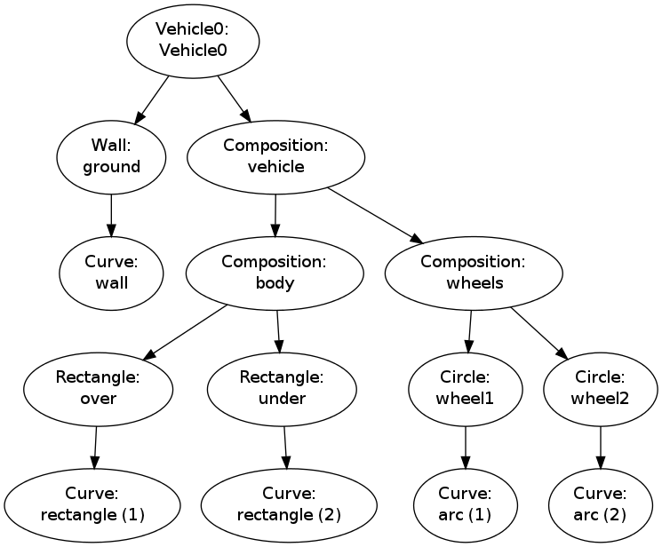
Let us follow a v.recurse('vehicle') call in detail, v being a Vehicle0 instance. Before looking into the output from recurse, let us get an overview of the figure hierarchy in the v object (as produced by print v)

ground
    wall
vehicle
    body
        over
            rectangle
        under
            rectangle
    wheels
        wheel1
            arc
        wheel2
            arc

The recurse method performs the same kind of traversal of the hierarchy, but writes out and explains a lot more.

The data structure represented by v.shapes is known as a tree. As in physical trees, there is a root, here the v.shapes dictionary. A graphical illustration of the tree (upside down) is shown in Figure 11. From the root there are one or more branches, here two: ground and vehicle. Following the vehicle branch, it has two new branches, body and wheels. Relationships as in family trees are often used to describe the relations in object trees too: we say that vehicle is the parent of body and that body is a child of vehicle. The term node is also often used to describe an element in a tree. A node may have several other nodes as descendants.

Figure 11: Hierarchy of figure elements in an instance of class Vehicle0.

Recursion is the principal programming technique to traverse tree structures. Any object in the tree can be viewed as a root of a subtree. For example, wheels is the root of a subtree that branches into wheel1 and wheel2. So when processing an object in the tree, we imagine we process the root and then recurse into a subtree, but the first object we recurse into can be viewed as the root of the subtree, so the processing procedure of the parent object can be repeated.

A recommended next step is to simulate the recurse method by hand and carefully check that what happens in the visits to recurse is consistent with the output listed below. Although tedious, this is a major exercise that guaranteed will help to demystify recursion.

A part of the printout of v.recurse('vehicle') looks like

 Vehicle0: vehicle.shapes has entries 'ground', 'vehicle'
 call vehicle.shapes["ground"].recurse("ground", 2)
   Wall: ground.shapes has entries 'wall'
   call ground.shapes["wall"].recurse("wall", 4)
     reached "bottom" object Curve
 call vehicle.shapes["vehicle"].recurse("vehicle", 2)
   Composition: vehicle.shapes has entries 'body', 'wheels'
   call vehicle.shapes["body"].recurse("body", 4)
     Composition: body.shapes has entries 'over', 'under'
     call body.shapes["over"].recurse("over", 6)
       Rectangle: over.shapes has entries 'rectangle'
       call over.shapes["rectangle"].recurse("rectangle", 8)
         reached "bottom" object Curve
     call body.shapes["under"].recurse("under", 6)
       Rectangle: under.shapes has entries 'rectangle'
       call under.shapes["rectangle"].recurse("rectangle", 8)
         reached "bottom" object Curve
...

This example should clearly demonstrate the principle that we can start at any object in the tree and do a recursive set of calls with that object as root.

Scaling, translating, and rotating a figure

With recursion, as explained in the previous section, we can within minutes equip all classes in the Shape hierarchy, both present and future ones, with the ability to scale the figure, translate it, or rotate it. This added functionality requires only a few lines of code.

Scaling

We start with the simplest of the three geometric transformations, namely scaling. For a Curve instance containing a set of $ n $ coordinates $ (x_i,y_i) $ that make up a curve, scaling by a factor $ a $ means that we multiply all the $ x $ and $ y $ coordinates by $ a $: $$ x_i \leftarrow ax_i,\quad y_i\leftarrow ay_i, \quad i=0,\ldots,n-1\thinspace . $$ Here we apply the arrow as an assignment operator. The corresponding Python implementation in class Curve reads

class Curve:
    ...
    def scale(self, factor):
        self.x = factor*self.x
        self.y = factor*self.y

Note here that self.x and self.y are Numerical Python arrays, so that multiplication by a scalar number factor is a vectorized operation.

An even more efficient implementation is to make use of in-place multiplication in the arrays,

class Curve:
    ...
    def scale(self, factor):
        self.x *= factor
        self.y *= factor

as this saves the creation of temporary arrays like factor*self.x.

In an instance of a subclass of Shape, the meaning of a method scale is to run through all objects in the dictionary shapes and ask each object to scale itself. This is the same delegation of actions to subclass instances as we do in the draw (or recurse) method. All objects, except Curve instances, can share the same implementation of the scale method. Therefore, we place the scale method in the superclass Shape such that all subclasses inherit the method. Since scale and draw are so similar, we can easily implement the scale method in class Shape by copying and editing the draw method:

class Shape:
    ...
    def scale(self, factor):
        for shape in self.shapes:
            self.shapes[shape].scale(factor)

This is all we have to do in order to equip all subclasses of Shape with scaling functionality! Any piece of the figure will scale itself, in the same manner as it can draw itself.

Translation

A set of coordinates $ (x_i, y_i) $ can be translated $ v_0 $ units in the $ x $ direction and $ v_1 $ units in the $ y $ direction using the formulas $$ \begin{equation*} x_i\leftarrow x_i+v_0,\quad y_i\leftarrow y_i+v_1, \quad i=0,\ldots,n-1\thinspace . \end{equation*} $$ The natural specification of the translation is in terms of the vector $ v=(v_0,v_1) $. The corresponding Python implementation in class Curve becomes

class Curve:
    ...
    def translate(self, v):
        self.x += v[0]
        self.y += v[1]

The translation operation for a shape object is very similar to the scaling and drawing operations. This means that we can implement a common method translate in the superclass Shape. The code is parallel to the scale method:

class Shape:
    ....
    def translate(self, v):
        for shape in self.shapes:
            self.shapes[shape].translate(v)

Rotation

Rotating a figure is more complicated than scaling and translating. A counter clockwise rotation of $ \theta $ degrees for a set of coordinates $ (x_i,y_i) $ is given by $$ \begin{align*} \bar x_i &\leftarrow x_i\cos\theta - y_i\sin\theta,\\ \bar y_i &\leftarrow x_i\sin\theta + y_i\cos\theta\thinspace . \end{align*} $$ This rotation is performed around the origin. If we want the figure to be rotated with respect to a general point $ (x,y) $, we need to extend the formulas above: $$ \begin{align*} \bar x_i &\leftarrow x + (x_i -x)\cos\theta - (y_i -y)\sin\theta,\\ \bar y_i &\leftarrow y + (x_i -x)\sin\theta + (y_i -y)\cos\theta\thinspace . \end{align*} $$ The Python implementation in class Curve, assuming that $ \theta $ is given in degrees and not in radians, becomes

    def rotate(self, angle, center):
        angle = radians(angle)
        x, y = center
        c = cos(angle);  s = sin(angle)
        xnew = x + (self.x - x)*c - (self.y - y)*s
        ynew = y + (self.x - x)*s + (self.y - y)*c
        self.x = xnew
        self.y = ynew

The rotate method in class Shape follows the principle of the draw, scale, and translate methods.

We have already seen the rotate method in action when animating the rolling wheel at the end of the section Animation: rolling the wheels.