A simple pendulum
The basic physics sketch
We now want to make a sketch of simple pendulum from physics, as shown in Figure 8. A body with mass \( m \) is attached to a massless, stiff rod, which can rotate about a point, causing the pendulum to oscillate.
A suggested work flow is to
first sketch the figure on a piece of paper and introduce a coordinate
system. A simple coordinate system is indicated in Figure
9. In a code we introduce variables
W and H for the width and height of the figure (i.e., extent of
the coordinate system) and open the program like this:
from pysketcher import *

H = 7.
W = 6.

drawing_tool.set_coordinate_system(xmin=0, xmax=W,
                                   ymin=0, ymax=H,
                                   axis=True)
drawing_tool.set_grid(True)
drawing_tool.set_linecolor('blue')
Note that when the sketch is ready for "production", we will (normally)
set axis=False to remove the coordinate system and also remove the
grid, i.e., delete or
comment out the line drawing_tool.set_grid(True).
Also note that we in this example let all lines be blue by default.
Figure 8: Sketch of a simple pendulum.
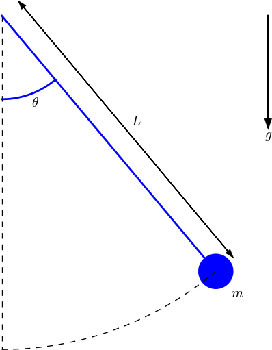
Figure 9: Sketch with assisting coordinate system.
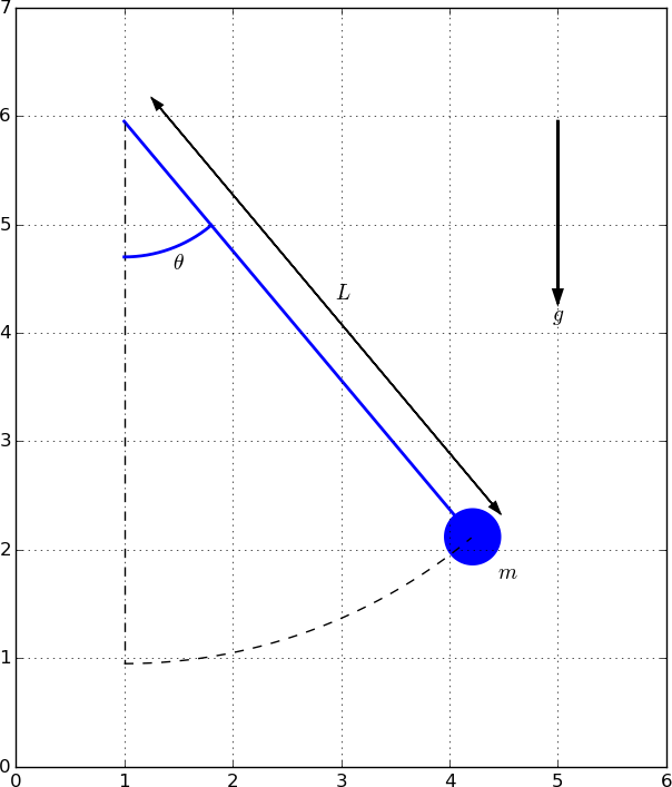
The next step is to introduce variables for key quantities in the sketch.
Let L be the length of the pendulum, P the rotation point, and let
a be the angle the pendulum makes with the vertical (measured in degrees).
We may set
L = 5*H/7          # length
P = (W/6, 0.85*H)  # rotation point
a = 40             # angle
Be careful with integer division if you use Python 2! Fortunately, we
started out with float objects for W and H so the expressions above
are safe.
What kind of objects do we need in this sketch? Looking at Figure 8 we see that we need
- a vertical, dashed line
- an arc with no text but dashed line to indicate the path of the mass
- an arc with name \( \theta \) to indicate the angle
- a line, here called rod, from the rotation point to the mass
- a blue, filled circle representing the mass
- a text \( m \) associated with the mass
- an indicator of the pendulum's length \( L \), visualized as a line with two arrows tips and the text \( L \)
- a gravity vector with the text \( g \)
P to P minus the length \( L \) in \( y \) direction:
vertical = Line(P, P-point(0,L))
The class point is very convenient: it turns its two coordinates into
a vector with which we can compute, and is therefore one of the most
widely used Pysketcher objects.
The path of the mass is an arc that can be made by
Pysketcher's Arc object:
path = Arc(P, L, -90, a)
The first argument P is the center point, the second is the
radius (L here), the next argument is the start angle, here
it starts at -90 degrees, while the next argument is the angle of
the arc, here a.
For the path of the mass, we also need an arc object, but this
time with an associated text. Pysketcher has a specialized object
for this purpose, Arc_wText, since placing the text manually can
be somewhat cumbersome.
angle = Arc_wText(r'$\theta$', P, L/4, -90, a, text_spacing=1/30.)
The arguments are as for Arc above, but the first one is the desired
text. Remember to use a raw string since we want a LaTeX greek letter
that contains a backslash.
The text_spacing argument must often be tweaked. It is recommended
to create only a few objects before rendering the sketch and then
adjust spacings as one goes along.
The rod is simply a line from P to the mass. We can easily
compute the position of the mass from basic geometry considerations,
but it is easier and safer to look up this point in other objects
if it is already computed. In the present case,
the path object stored its start and
end points, so path.geometric_features()['end'] is the end point
of the path, which is the position of the mass. We can therefore
create the rod simply as a line from P to this already computed end point:
mass_pt = path.geometric_features()['end']
rod = Line(P, mass_pt)
The mass is a circle filled with color:
mass = Circle(center=mass_pt, radius=L/20.)
mass.set_filled_curves(color='blue')
To place the \( m \) correctly, we go a small distance in the direction of
the rod, from the center of the circle. To this end, we need to
compute the direction. This is easiest done by computing a vector
from P to the center of the circle and calling unit_vec to make
a unit vector in this direction:
rod_vec = rod.geometric_features()['end'] - \
          rod.geometric_features()['start']
unit_rod_vec = unit_vec(rod_vec)
mass_symbol = Text('$m$', mass_pt + L/10*unit_rod_vec)
Again, the distance L/10 is something one has to experiment with.
The next object is the length measure with the text \( L \). Such length
measures are represented by Pysketcher's Distance_wText object.
An easy construction is to first place this length measure along the
rod and then translate it a little distance (L/15) in the
normal direction of the rod:
length = Distance_wText(P, mass_pt, '$L$')
length.translate(L/15*point(cos(radians(a)), sin(radians(a))))
For this translation we need a unit vector in the normal direction
of the rod, which is from geometric considerations given by
\( (\cos a, \sin a) \), when \( a \) is the angle of the pendulum.
Alternatively, we could have found the normal vector as a vector that
is normal to unit_rod_vec: point(-unit_rod_vec[1],unit_rod_vec[0]).
The final object is the gravity force vector, which is so common
in physics sketches that Pysketcher has a ready-made object: Gravity,
gravity = Gravity(start=P+point(0.8*L,0), length=L/3)
Since blue is the default color for
lines, we want the dashed lines (for vertical and path) to be black
and with linewidth 1. These properties can be set one by one for each
object, but we can also make a little helper function:
def set_dashed_thin_blackline(*objects):
    """Set linestyle of objects to dashed, black, width=1."""
    for obj in objects:
        obj.set_linestyle('dashed')
        obj.set_linecolor('black')
        obj.set_linewidth(1)

set_dashed_thin_blackline(vertical, path)
Now, all objects are in place, so it remains to compose the final figure and draw the composition:
fig = Composition(
    {'body': mass, 'rod': rod,
     'vertical': vertical, 'theta': angle, 'path': path,
     'g': gravity, 'L': length, 'm': mass_symbol})

fig.draw()
drawing_tool.display()
drawing_tool.savefig('pendulum1')
The body diagram
Now we want to isolate the mass and draw all the forces that act on it. Figure 10 shows the desired result, but embedded in the coordinate system. We consider three types of forces: the gravity force, the force from the rod, and air resistance. The body diagram is key for deriving the equation of motion, so it is illustrative to add useful mathematical quantities needed in the derivation, such as the unit vectors in polar coordinates.
Figure 10: Body diagram of a simple pendulum.
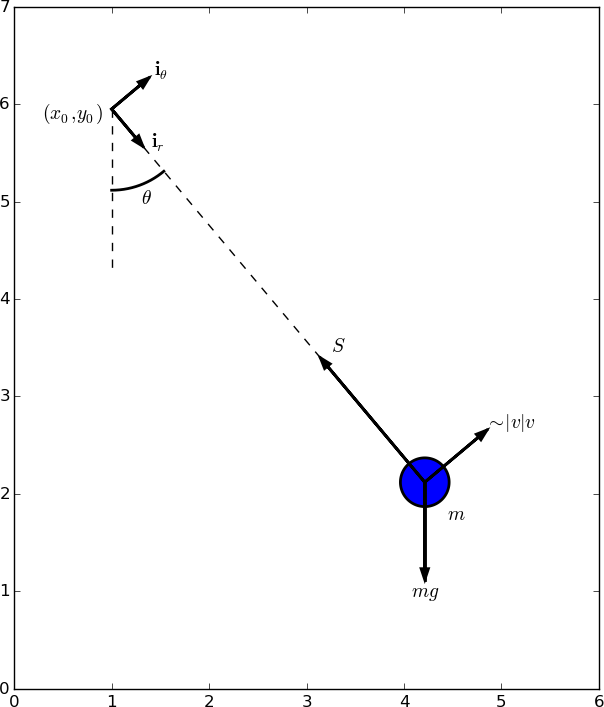
We start by listing the objects in the sketch:
- a text \( (x_0,y_0) \) representing the rotation point
P - unit vector \( \boldsymbol{i}_r \) with text
- unit vector \( \boldsymbol{i}_\theta \) with text
- a dashed vertical line
- a dashed line along the rod
- an arc with text \( \theta \)
- the gravity force with text \( mg \)
- the force in the rod with text \( S \)
- the air resistance force with text \( \sim |v|v \)
Force object since it has an
arrow with a text. The first three objects can then be made as follows:
x0y0 = Text('$(x_0,y_0)$', P + point(-0.4,-0.1))
ir = Force(P, P + L/10*unit_vec(rod_vec),
           r'$\boldsymbol{i}_r$', text_pos='end',
           text_spacing=(0.015,0))
ith = Force(P, P + L/10*unit_vec((-rod_vec[1], rod_vec[0])),
           r'$\boldsymbol{i}_{\theta}$', text_pos='end',
            text_spacing=(0.02,0.005))
Note that tweaking of the position of x0y0 use absolute coordinates, so
if W or H is changed in the beginning of the figure, the tweaked position
will most likely not look good. A better solution would be to express
the tweaked displacement point(-0.4,-0.1) in terms of W and H.
The text_spacing values in the Force objects also use absolute
coordinates. Very often, this is much more convenient when adjusting
the objects, and global size parameters like W and H are in practice
seldom changed, so the solution above is quite typical.
The vertical, dashed line, the dashed rod, and the arc for \( \theta \) are made by
rod_start = rod.geometric_features()['start']  # Point P
vertical2 = Line(rod_start, rod_start + point(0,-L/3))
set_dashed_thin_blackline(vertical2)
set_dashed_thin_blackline(rod)
angle2 = Arc_wText(r'$\theta$', rod_start, L/6, -90, a,
                   text_spacing=1/30.)
Note how we reuse the earlier defined object rod.
The forces are constructed as shown below.
mg_force  = Force(mass_pt, mass_pt + L/5*point(0,-1),
                  '$mg$', text_pos='end')
rod_force = Force(mass_pt, mass_pt - L/3*unit_vec(rod_vec),
                  '$S$', text_pos='end',
                  text_spacing=(0.03, 0.01))
air_force = Force(mass_pt, mass_pt -
                  L/6*unit_vec((rod_vec[1], -rod_vec[0])),
                  '$\sim|v|v$', text_pos='end',
                  text_spacing=(0.04,0.005))
Note that the drag force from the air is directed perpendicular to
the rod, so we construct a unit vector in this direction directly from
the rod_vec vector.
All objects are in place, and we can compose a figure to be drawn:
body_diagram = Composition(
    {'mg': mg_force, 'S': rod_force, 'rod': rod,
     'vertical': vertical2, 'theta': angle2,
     'body': mass, 'm': mass_symbol})

body_diagram['air'] = air_force
body_diagram['ir'] = ir
body_diagram['ith'] = ith
body_diagram['origin'] = x0y0
Here, we exemplify that we can start out with a composition as a dictionary, but (as in ordinary Python dictionaries) add new elements later when desired.
Animated body diagram
We want to make an animated body diagram so that we can see how forces develop in time according to the motion. This means that we must couple the sketch at each time level to a numerical solution for the motion of the pendulum.
Function for drawing the body diagram
The previous flat program for making sketches of the pendulum is not suitable when we want to make a sketch at a lot of different points in time, i.e., for a lot of different angles that the pendulum makes with the vertical. We therefore need to draw the body diagram in a function where the angle is a parameter. We also supply arrays containing the (numerically computed) values of the angle \( \theta \) and the forces at various time levels, plus the desired time point and level for this particular sketch:
from pysketcher import *

H = 15.
W = 17.

drawing_tool.set_coordinate_system(xmin=0, xmax=W,
                                   ymin=0, ymax=H,
                                   axis=False)

def pendulum(theta, S, mg, drag, t, time_level):

    drawing_tool.set_linecolor('blue')
    import math
    a = math.degrees(theta[time_level])
    L = 0.4*H         # length
    P = (W/2, 0.8*H)  # rotation point

    vertical = Line(P, P-point(0,L))
    path = Arc(P, L, -90, a)
    angle = Arc_wText(r'$\theta$', P, L/4, -90, a, text_spacing=1/30.)

    mass_pt = path.geometric_features()['end']
    rod = Line(P, mass_pt)

    mass = Circle(center=mass_pt, radius=L/20.)
    mass.set_filled_curves(color='blue')
    rod_vec = rod.geometric_features()['end'] - \
              rod.geometric_features()['start']
    unit_rod_vec = unit_vec(rod_vec)
    mass_symbol = Text('$m$', mass_pt + L/10*unit_rod_vec)

    length = Distance_wText(P, mass_pt, '$L$')
    # Displace length indication
    length.translate(L/15*point(cos(radians(a)), sin(radians(a))))
    gravity = Gravity(start=P+point(0.8*L,0), length=L/3)

    def set_dashed_thin_blackline(*objects):
        """Set linestyle of objects to dashed, black, width=1."""
        for obj in objects:
            obj.set_linestyle('dashed')
            obj.set_linecolor('black')
            obj.set_linewidth(1)

    set_dashed_thin_blackline(vertical, path)

    fig = Composition(
        {'body': mass, 'rod': rod,
         'vertical': vertical, 'theta': angle, 'path': path,
         'g': gravity, 'L': length})

    #fig.draw()
    #drawing_tool.display()
    #drawing_tool.savefig('tmp_pendulum1')

    drawing_tool.set_linecolor('black')

    rod_start = rod.geometric_features()['start']  # Point P
    vertical2 = Line(rod_start, rod_start + point(0,-L/3))
    set_dashed_thin_blackline(vertical2)
    set_dashed_thin_blackline(rod)
    angle2 = Arc_wText(r'$\theta$', rod_start, L/6, -90, a,
                       text_spacing=1/30.)

    magnitude = 1.2*L/2   # length of a unit force in figure
    force = mg[time_level]  # constant (scaled eq: about 1)
    force *= magnitude
    mg_force  = Force(mass_pt, mass_pt + force*point(0,-1),
                      '', text_pos='end')
    force = S[time_level]
    force *= magnitude
    rod_force = Force(mass_pt, mass_pt - force*unit_vec(rod_vec),
                      '', text_pos='end',
                      text_spacing=(0.03, 0.01))
    force = drag[time_level]
    force *= magnitude
    #print('drag(%g)=%g' % (t, drag[time_level]))
    air_force = Force(mass_pt, mass_pt -
                      force*unit_vec((rod_vec[1], -rod_vec[0])),
                      '', text_pos='end',
                      text_spacing=(0.04,0.005))

    body_diagram = Composition(
        {'mg': mg_force, 'S': rod_force, 'air': air_force,
         'rod': rod,
         'vertical': vertical2, 'theta': angle2,
         'body': mass})

    x0y0 = Text('$(x_0,y_0)$', P + point(-0.4,-0.1))
    ir = Force(P, P + L/10*unit_vec(rod_vec),
               r'$\boldsymbol{i}_r$', text_pos='end',
               text_spacing=(0.015,0))
    ith = Force(P, P + L/10*unit_vec((-rod_vec[1], rod_vec[0])),
               r'$\boldsymbol{i}_{\theta}$', text_pos='end',
                text_spacing=(0.02,0.005))

    #body_diagram['ir'] = ir
    #body_diagram['ith'] = ith
    #body_diagram['origin'] = x0y0

    drawing_tool.erase()
    body_diagram.draw(verbose=0)
    #drawing_tool.display('Body diagram')
    drawing_tool.savefig('tmp_%04d.png' % time_level, crop=False)
    # No cropping: otherwise movies will be very strange
Equations for the motion and forces
The modeling of the motion of a pendulum is most conveniently done in polar coordinates since then the unknown force in the rod is separated from the equation determining the motion \( \theta(t) \). The position vector for the mass is $$ \rpos = x_0\ii + y_0\jj + L\ir\tp$$ The corresponding acceleration becomes $$ \ddot{\rpos} = L\ddot{\theta}{\ith} - L\dot{\theta^2}{\ir}\tp$$
There are three forces on the mass: the gravity force \( mg\jj = mg(-\cos\theta\,\ir + \sin\theta\,\ith) \), the force in the rod \( -S\ir \), and the drag force because of air resistance: $$ -\half C_D \varrho \pi R^2 |v|v\,\ith,$$ where \( C_D\approx 0.4 \) is the drag coefficient for a sphere, \( \varrho \) is the density of air, \( R \) is the radius of the mass, and \( v \) is the velocity (\( v=L\dot\theta \)). The drag force acts in \( -\ith \) direction when \( v>0 \).
Newton's second law of motion for the pendulum now becomes $$ mL\ddot\theta\ith - mL\dot\theta^2\ir = -mg(-\cos\theta\,\ir + \sin\theta\,\ith) -S\ir - \half C_D \varrho \pi R^2 L^2|\dot\theta|\dot\theta\ith,$$ which gives two component equations $$ \begin{align} mL\ddot\theta + \half C_D \varrho \pi R^2 L^2|\dot\theta|\dot\theta + mg\sin\theta &= 0, \tag{1}\\ S &= mL\dot\theta^2 + mg\cos\theta \tag{2}\tp \end{align} $$
It is almost always convenient to scale such equations. Introducing the dimensionless time $$ \bar t = \frac{t}{t_c},\quad t_c = \sqrt{\frac{L}{g}},$$ leads to $$ \begin{align} \frac{d^2\theta}{d\bar t^2} + \alpha\left\vert\frac{d\theta}{d\bar t}\right\vert\frac{d\theta}{d\bar t} + \sin\theta &= 0, \tag{3}\\ \bar S &= \left(\frac{d\theta}{d\bar t}\right)^2 + \cos\theta, \tag{4} \end{align} $$ where \( \alpha \) is a dimensionless drag coefficient $$ \alpha = \frac{C_D\varrho\pi R^2L}{2m},$$ and \( \bar S \) is the scaled force $$ \bar S = \frac{S}{mg}\tp$$ We see that \( \bar S = 1 \) for the equilibrium position \( \theta=0 \), so this scaling of \( S \) seems appropriate.
The parameter \( \alpha \) is about the ratio of the drag force and the gravity force: $$ \frac{|\half C_D\varrho \pi R^2 |v|v|}{|mg|}\sim \frac{C_D\varrho \pi R^2 L^2 t_c^{-2}}{mg} \left|\frac{d\bar\theta}{d\bar t}\right|\frac{d\bar\theta}{d\bar t} \sim \frac{C_D\varrho \pi R^2 L}{2m}\theta_0^2 = \alpha \theta_0^2\tp$$ (We have that \( \theta(t)/d\theta_0 \) is in \( [-1,1] \), so we expect since \( \theta_0^{-1}d\bar\theta/d\bar t \) to be around unity. Here, \( \theta_0=\theta(0) \).)
The next step is to write a numerical solver for (3)-(4). To this end, we use the Odespy package. The system of second-order ODEs must be expressed as a system of first-order ODEs. We realize that the unknown \( \bar S \) is decoupled from \( \theta \) in the sense that we can first use (3) to solve for \( \theta \) and then compute \( \bar S \) from (4). The first-order ODEs become $$ \begin{align} \frac{d\omega}{d\bar t} &= -\alpha\left\vert\omega\right\vert\omega - \sin\theta, \tag{5}\\ \frac{d\theta}{d\bar t} &= \omega\tp \tag{6} \end{align} $$ Then we compute $$ \begin{equation} \bar S = \omega^2 + \cos\theta\tp \tag{7} \end{equation} $$ The dimensionless air resistance force can also be computed: $$ \begin{equation} -\alpha|\omega|\omega\tp \tag{8} \end{equation} $$ Since we scaled the force \( S \) by \( mg \), \( mg \) is the natural force scale, and the \( mg \) force itself is then unity.
By updating \( \omega \) in the first equation, we can use an Euler-Cromer scheme on Odespy (all other schemes are independent of whether the \( \theta \) or \( \omega \) equation comes first).
Numerical solution
An appropriate solver is
def simulate_pendulum(alpha, theta0, dt, T):
    import odespy

    def f(u, t, alpha):
        omega, theta = u
        return [-alpha*omega*abs(omega) - sin(theta),
                omega]

    import numpy as np
    Nt = int(round(T/float(dt)))
    t = np.linspace(0, Nt*dt, Nt+1)
    solver = odespy.RK4(f, f_args=[alpha])
    solver.set_initial_condition([0, theta0])
    u, t = solver.solve(t,
                        terminate=lambda u, t, n: abs(u[n,1]) < 1E-3)
    omega = u[:,0]
    theta = u[:,1]
    S = omega**2 + np.cos(theta)
    drag = -alpha*np.abs(omega)*omega
    return t, theta, omega, S, drag
Animation
We can finally traverse the time array and draw a body diagram
at each time level. The resulting sketches are saved to files
tmp_%04d.png, and these files can be combined to videos:
def animate():
    # Clean up old plot files
    import os, glob
    for filename in glob.glob('tmp_*.png') + glob.glob('movie.*'):
        os.remove(filename)
    # Solve problem
    from math import pi, radians, degrees
    import numpy as np
    alpha = 0.4
    period = 2*pi
    T = 12*period
    dt = period/40
    a = 70
    theta0 = radians(a)
    t, theta, omega, S, drag = simulate_pendulum(alpha, theta0, dt, T)
    mg = np.ones(S.size)
    # Visualize drag force 5 times as large
    drag *= 5
    print('NOTE: drag force magnified 5 times!!')

    # Draw animation
    import time
    for time_level, t_ in enumerate(t):
        pendulum(theta, S, mg, drag, t_, time_level)
        time.sleep(0.2)

    # Make videos
    prog = 'ffmpeg'
    filename = 'tmp_%04d.png'
    fps = 6
    codecs = {'flv': 'flv', 'mp4': 'libx264',
              'webm': 'libvpx', 'ogg': 'libtheora'}
    for ext in codecs:
        lib = codecs[ext]
        cmd = '%(prog)s -i %(filename)s -r %(fps)s ' % vars()
        cmd += '-vcodec %(lib)s movie.%(ext)s' % vars()
        print(cmd)
        os.system(cmd)
This time we did not use the animate function from Pysketcher, but
stored each sketch in a file with drawing_tool.savefig. Note that
the argument crop=False is key: otherwise each figure is cropped and
it makes to sense to combine the images to a video. By default,
Pysketcher crops (removes all exterior whitespace) from figures saved
to file.
The drag force is magnified 5 times (compared to \( mg \) and \( S \)!