A first glimpse of Pysketcher
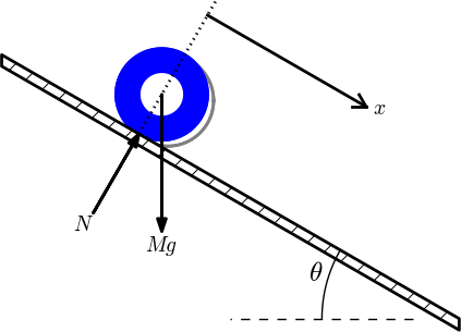
Formulation of physical problems makes heavy use of principal sketches such as the one in Figure 1. This particular sketch illustrates the classical mechanics problem of a rolling wheel on an inclined plane. The figure is made up many individual elements: a rectangle filled with a pattern (the inclined plane), a hollow circle with color (the wheel), arrows with labels (the \( N \) and \( Mg \) forces, and the \( x \) axis), an angle with symbol \( \theta \), and a dashed line indicating the starting location of the wheel.
Drawing software and plotting programs can produce such figures quite easily in principle, but the amount of details the user needs to control with the mouse can be substantial. Software more tailored to producing sketches of this type would work with more convenient abstractions, such as circle, wall, angle, force arrow, axis, and so forth. And as soon we start programming to construct the figure we get a range of other powerful tools at disposal. For example, we can easily translate and rotate parts of the figure and make an animation that illustrates the physics of the problem. Programming as a superior alternative to interactive drawing is the mantra of this section.
Figure 1: Sketch of a physics problem.
Basic construction of sketches
Before attacking real-life sketches as in Figure 1 we focus on the significantly simpler drawing shown in Figure 2. This toy sketch consists of several elements: two circles, two rectangles, and a "ground" element.
Figure 2: Sketch of a simple figure.
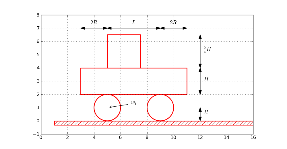
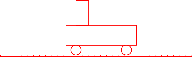
When the sketch is defined in terms of computer code, it is natural to parameterize geometric features, such as the radius of the wheel (\( R \)), the center point of the left wheel (\( w_1 \)), as well as the height (\( H \)) and length (\( L \)) of the main part. The simple vehicle in Figure 2 is quickly drawn in almost any interactive tool. However, if we want to change the radius of the wheels, you need a sophisticated drawing tool to avoid redrawing the whole figure, while in computer code this is a matter of changing the \( R \) parameter and rerunning the program. For example, Figure 3 shows a variation of the drawing in Figure 2 obtained by just setting \( R=0.5 \), \( L=5 \), \( H=2 \), and \( R=2 \). Being able to quickly change geometric sizes is key to many problem settings in physics and engineering, but then a program must define the geometry.
Figure 3: Redrawing a figure with other geometric parameters.
Basic drawing
A typical program creating these five elements is shown next.
After importing the pysketcher package, the first task is always to
define a coordinate system:
from pysketcher import *

drawing_tool.set_coordinate_system(
    xmin=0, xmax=10, ymin=-1, ymax=8)
Instead of working with lengths expressed by specific numbers it is highly recommended to use variables to parameterize lengths as this makes it easier to change dimensions later. Here we introduce some key lengths for the radius of the wheels, distance between the wheels, etc.:
R = 1    # radius of wheel
L = 4    # distance between wheels
H = 2    # height of vehicle body
w_1 = 5  # position of front wheel
drawing_tool.set_coordinate_system(xmin=0, xmax=w_1 + 2*L + 3*R,
                                   ymin=-1, ymax=2*R + 3*H)
With the drawing area in place we can make the first Circle object
in an intuitive fashion:
wheel1 = Circle(center=(w_1, R), radius=R)
to change dimensions later.
To translate the geometric information about the wheel1 object to
instructions for the plotting engine (in this case Matplotlib), one calls the
wheel1.draw(). To display all drawn objects, one issues
drawing_tool.display(). The typical steps are hence:
wheel1 = Circle(center=(w_1, R), radius=R)
wheel1.draw()

# Define other objects and call their draw() methods
drawing_tool.display()
drawing_tool.savefig('tmp.png')  # store picture
The next wheel can be made by taking a copy of wheel1 and
translating the object to the right according to a
displacement vector \( (L,0) \):
wheel2 = wheel1.copy()
wheel2.translate((L,0))
The two rectangles are also made in an intuitive way:
under = Rectangle(lower_left_corner=(w_1-2*R, 2*R),
                  width=2*R + L + 2*R, height=H)
over  = Rectangle(lower_left_corner=(w_1, 2*R + H),
                  width=2.5*R, height=1.25*H)
Groups of objects
Instead of calling the draw method of every object, we can
group objects and call draw, or perform other operations, for
the whole group. For example, we may collect the two wheels
in a wheels group and the over and under rectangles
in a body group. The whole vehicle is a composition
of its wheels and body groups. The code goes like
wheels  = Composition({'wheel1': wheel1, 'wheel2': wheel2})
body    = Composition({'under': under, 'over': over})

vehicle = Composition({'wheels': wheels, 'body': body})
The ground is illustrated by an object of type Wall,
mostly used to indicate walls in sketches of mechanical systems.
A Wall takes the x and y coordinates of some curve,
and a thickness parameter, and creates a thick curve filled
with a simple pattern. In this case the curve is just a flat
line so the construction is made of two points on the
ground line (\( (w_1-L,0) \) and \( (w_1+3L,0) \)):
ground = Wall(x=[w_1 - L, w_1 + 3*L], y=[0, 0], thickness=-0.3*R)
The negative thickness makes the pattern-filled rectangle appear below the defined line, otherwise it appears above.
We may now collect all the objects in a "top" object that contains the whole figure:
fig = Composition({'vehicle': vehicle, 'ground': ground})
fig.draw()  # send all figures to plotting backend
drawing_tool.display()
drawing_tool.savefig('tmp.png')
The fig.draw() call will visit
all subgroups, their subgroups,
and so forth in the hierarchical tree structure of
figure elements,
and call draw for every object.
Changing line styles and colors
Controlling the line style, line color, and line width is
fundamental when designing figures. The pysketcher
package allows the user to control such properties in
single objects, but also set global properties that are
used if the object has no particular specification of
the properties. Setting the global properties are done like
drawing_tool.set_linestyle('dashed')
drawing_tool.set_linecolor('black')
drawing_tool.set_linewidth(4)
At the object level the properties are specified in a similar way:
wheels.set_linestyle('solid')
wheels.set_linecolor('red')
and so on.
Geometric figures can be specified as filled, either with a color or with a special visual pattern:
# Set filling of all curves
drawing_tool.set_filled_curves(color='blue', pattern='/')

# Turn off filling of all curves
drawing_tool.set_filled_curves(False)

# Fill the wheel with red color
wheel1.set_filled_curves('red')
The figure composition as an object hierarchy
The composition of objects making up the figure
is hierarchical, similar to a family, where
each object has a parent and a number of children. Do a
print fig to display the relations:
ground
    wall
vehicle
    body
        over
            rectangle
        under
            rectangle
    wheels
        wheel1
            arc
        wheel2
            arc
The indentation reflects how deep down in the hierarchy (family) we are. This output is to be interpreted as follows:
-
figcontains two objects,groundandvehicle -
groundcontains an objectwall -
vehiclecontains two objects,bodyandwheels -
bodycontains two objects,overandunder -
wheelscontains two objects,wheel1andwheel2
rectangle and arc. These are of type Curve
and automatically generated by the classes Rectangle and Circle.
More detailed information can be printed by
print fig.show_hierarchy('std')
yielding the output
ground (Wall):
    wall (Curve): 4 coords fillcolor='white' fillpattern='/'
vehicle (Composition):
    body (Composition):
        over (Rectangle):
            rectangle (Curve): 5 coords
        under (Rectangle):
            rectangle (Curve): 5 coords
    wheels (Composition):
        wheel1 (Circle):
            arc (Curve): 181 coords
        wheel2 (Circle):
            arc (Curve): 181 coords
Here we can see the class type for each figure object, how many
coordinates that are involved in basic figures (Curve objects), and
special settings of the basic figure (fillcolor, line types, etc.).
For example, wheel2 is a Circle object consisting of an arc,
which is a Curve object consisting of 181 coordinates (the
points needed to draw a smooth circle). The Curve objects are the
only objects that really holds specific coordinates to be drawn.
The other object types are just compositions used to group
parts of the complete figure.
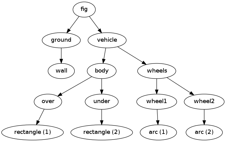
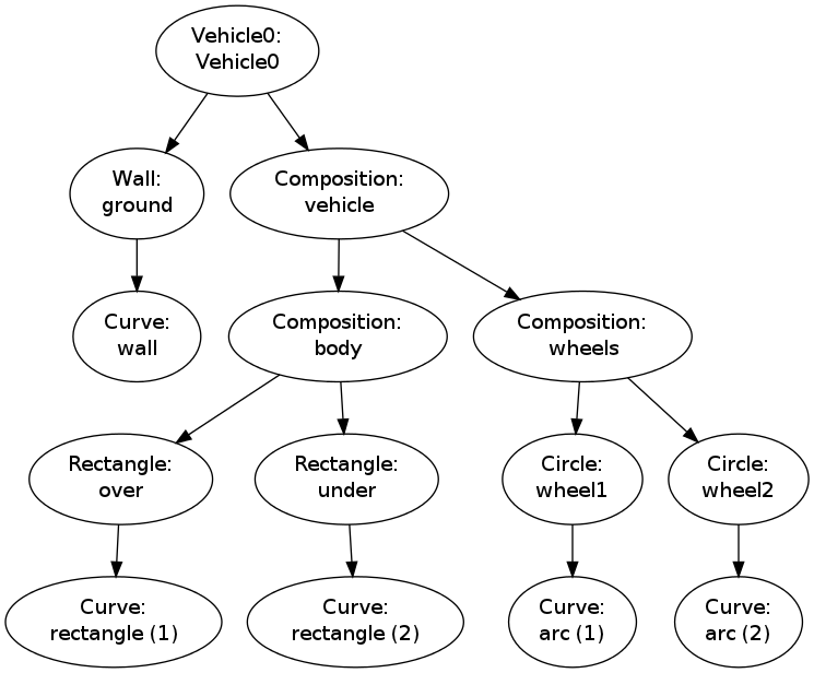
One can also get a graphical overview of the hierarchy of figure objects
that build up a particular figure fig.
Just call fig.graphviz_dot('fig') to produce a file fig.dot in
the dot format. This file contains relations between parent and
child objects in the figure and can be turned into an image,
as in Figure 4, by
running the dot program:
Terminal> dot -Tpng -o fig.png fig.dot
Figure 4: Hierarchical relation between figure objects.
The call fig.graphviz_dot('fig', classname=True) makes a fig.dot file
where the class type of each object is also visible, see
Figure 5. The ability to write out the
object hierarchy or view it graphically can be of great help when
working with complex figures that involve layers of subfigures.
Figure 5: Hierarchical relation between figure objects, including their class names.
Any of the objects can in the program be reached through their names, e.g.,
fig['vehicle']
fig['vehicle']['wheels']
fig['vehicle']['wheels']['wheel2']
fig['vehicle']['wheels']['wheel2']['arc']
fig['vehicle']['wheels']['wheel2']['arc'].x  # x coords
fig['vehicle']['wheels']['wheel2']['arc'].y  # y coords
fig['vehicle']['wheels']['wheel2']['arc'].linestyle
fig['vehicle']['wheels']['wheel2']['arc'].linetype
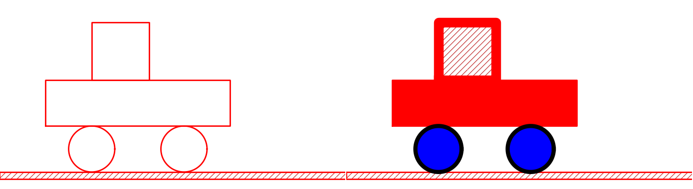
Grabbing a part of the figure this way is handy for changing properties of that part, for example, colors, line styles (see Figure 6):
fig['vehicle']['wheels'].set_filled_curves('blue')
fig['vehicle']['wheels'].set_linewidth(6)
fig['vehicle']['wheels'].set_linecolor('black')

fig['vehicle']['body']['under'].set_filled_curves('red')

fig['vehicle']['body']['over'].set_filled_curves(pattern='/')
fig['vehicle']['body']['over'].set_linewidth(14)
fig['vehicle']['body']['over']['rectangle'].linewidth = 4
The last line accesses the Curve object directly, while the line above,
accesses the Rectangle object, which will then set the linewidth of
its Curve object, and other objects if it had any.
The result of the actions above is shown in Figure 6.
Figure 6: Left: Basic line-based drawing. Right: Thicker lines and filled parts.
We can also change position of parts of the figure and thereby make animations, as shown next.
Animation: translating the vehicle
Can we make our little vehicle roll? A first attempt will be to
fake rolling by just displacing all parts of the vehicle.
The relevant parts constitute the fig['vehicle'] object.
This part of the figure can be translated, rotated, and scaled.
A translation along the ground means a translation in \( x \) direction,
say a length \( L \) to the right:
fig['vehicle'].translate((L,0))
You need to erase, draw, and display to see the movement:
drawing_tool.erase()
fig.draw()
drawing_tool.display()
Without erasing, the old drawing of the vehicle will remain in
the figure so you get two vehicles. Without fig.draw() the
new coordinates of the vehicle will not be communicated to
the drawing tool, and without calling display the updated
drawing will not be visible.
A figure that moves in time is conveniently realized by the
function animate:
animate(fig, tp, action)
Here, fig is the entire figure, tp is an array of
time points, and action is a user-specified function that changes
fig at a specific time point. Typically, action will move
parts of fig.
In the present case we can define the movement through a velocity
function v(t) and displace the figure v(t)*dt for small time
intervals dt. A possible velocity function is
def v(t):
    return -8*R*t*(1 - t/(2*R))
Our action function for horizontal displacements v(t)*dt becomes
def move(t, fig):
    x_displacement = dt*v(t)
    fig['vehicle'].translate((x_displacement, 0))
Since our velocity is negative for \( t\in [0,2R] \) the displacement is to the left.
The animate function will for each time point t in tp erase
the drawing, call action(t, fig), and show the new figure by
fig.draw() and drawing_tool.display().
Here we choose a resolution of the animation corresponding to
25 time points in the time interval \( [0,2R] \):
import numpy
tp = numpy.linspace(0, 2*R, 25)
dt = tp[1] - tp[0]  # time step

animate(fig, tp, move, pause_per_frame=0.2)
The pause_per_frame adds a pause, here 0.2 seconds, between
each frame in the animation.
We can also ask animate to store each frame in a file:
files = animate(fig, tp, move_vehicle, moviefiles=True,
                pause_per_frame=0.2)
The files variable, here 'tmp_frame_%04d.png',
is the printf-specification used to generate the individual
plot files. We can use this specification to make a video
file via ffmpeg (or avconv on Debian-based Linux systems such
as Ubuntu). Videos in the Flash and WebM formats can be created
by
Terminal> ffmpeg -r 12 -i tmp_frame_%04d.png -vcodec flv mov.flv
Terminal> ffmpeg -r 12 -i tmp_frame_%04d.png -vcodec libvpx mov.webm
An animated GIF movie can also be made using the convert program
from the ImageMagick software suite:
Terminal> convert -delay 20 tmp_frame*.png mov.gif
Terminal> animate mov.gif  # play movie
The delay between frames, in units of 1/100 s,
governs the speed of the movie.
To play the animated GIF file in a web page, simply insert
<img src="mov.gif"> in the HTML code.
The individual PNG frames can be directly played in a web browser by running
Terminal> scitools movie output_file=mov.html fps=5 tmp_frame*
or calling
from scitools.std import movie
movie(files, encoder='html', output_file='mov.html')
in Python. Load the resulting file mov.html into a web browser
to play the movie.
Try to run vehicle0.py and
then load mov.html into a browser, or play one of the mov.*
video files. Alternatively, you can view a ready-made movie.
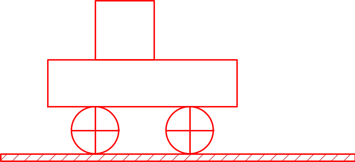
Animation: rolling the wheels
It is time to show rolling wheels. To this end, we add spokes to the wheels, formed by two crossing lines, see Figure 7. The construction of the wheels will now involve a circle and two lines:
wheel1 = Composition({
    'wheel': Circle(center=(w_1, R), radius=R),
    'cross': Composition({'cross1': Line((w_1,0),   (w_1,2*R)),
                          'cross2': Line((w_1-R,R), (w_1+R,R))})})
wheel2 = wheel1.copy()
wheel2.translate((L,0))
Observe that wheel1.copy() copies all the objects that make
up the first wheel, and wheel2.translate translates all
the copied objects.
Figure 7: Wheels with spokes to illustrate rolling.
The move function now needs to displace all the objects in the
entire vehicle and also rotate the cross1 and cross2
objects in both wheels.
The rotation angle follows from the fact that the arc length
of a rolling wheel equals the displacement of the center of
the wheel, leading to a rotation angle
angle = - x_displacement/R
With w_1 tracking the \( x \) coordinate of the center
of the front wheel, we can rotate that wheel by
w1 = fig['vehicle']['wheels']['wheel1']
from math import degrees
w1.rotate(degrees(angle), center=(w_1, R))
The rotate function takes two parameters: the rotation angle
(in degrees) and the center point of the rotation, which is the
center of the wheel in this case. The other wheel is rotated by
w2 = fig['vehicle']['wheels']['wheel2']
w2.rotate(degrees(angle), center=(w_1 + L, R))
That is, the angle is the same, but the rotation point is different.
The update of the center point is done by w_1 += x_displacement.
The complete move function with translation of the entire
vehicle and rotation of the wheels then becomes
w_1 = w_1 + L   # start position

def move(t, fig):
    x_displacement = dt*v(t)
    fig['vehicle'].translate((x_displacement, 0))

    # Rotate wheels
    global w_1
    w_1 += x_displacement
    # R*angle = -x_displacement
    angle = - x_displacement/R
    w1 = fig['vehicle']['wheels']['wheel1']
    w1.rotate(degrees(angle), center=(w_1, R))
    w2 = fig['vehicle']['wheels']['wheel2']
    w2.rotate(degrees(angle), center=(w_1 + L, R))
The complete example is found in the file vehicle1.py. You may run this file or watch a ready-made movie.
The advantages with making figures this way, through programming rather than using interactive drawing programs, are numerous. For example, the objects are parameterized by variables so that various dimensions can easily be changed. Subparts of the figure, possible involving a lot of figure objects, can change color, linetype, filling or other properties through a single function call. Subparts of the figure can be rotated, translated, or scaled. Subparts of the figure can also be copied and moved to other parts of the drawing area. However, the single most important feature is probably the ability to make animations governed by mathematical formulas or data coming from physics simulations of the problem, as shown in the example above.