Solving partial differential equations
The subject of partial differential equations (PDEs) is enormous. At the same time, it is very important, since so many phenomena in nature and technology find their mathematical formulation through such equations. Knowing how to solve at least some PDEs is therefore of great importance to engineers. In an introductory book like this, nowhere near full justice to the subject can be made. However, we still find it valuable to give the reader a glimpse of the topic by presenting a few basic and general methods that we will apply to a very common type of PDE.
We shall focus on one of the most widely encountered partial differential equations: the diffusion equation, which in one dimension looks like $$ \frac{\partial u}{\partial t} = \beta\frac{\partial^2 u}{\partial x^2} + g \thinspace .$$ The multi-dimensional counterpart is often written as $$ \frac{\partial u}{\partial t} = \beta\nabla^2 u + g \thinspace .$$ We shall restrict the attention here to the one-dimensional case.
The unknown in the diffusion equation is a function \( u(x,t) \) of space and time. The physical significance of \( u \) depends on what type of process that is described by the diffusion equation. For example, \( u \) is the concentration of a substance if the diffusion equation models transport of this substance by diffusion. Diffusion processes are of particular relevance at the microscopic level in biology, e.g., diffusive transport of certain ion types in a cell caused by molecular collisions. There is also diffusion of atoms in a solid, for instance, and diffusion of ink in a glass of water.
One very popular application of the diffusion equation is for heat transport in solid bodies. Then \( u \) is the temperature, and the equation predicts how the temperature evolves in space and time within the solid body. For such applications, the equations is known as the heat equation. We remark that the temperature in a fluid is influenced not only by diffusion, but also by the flow of the liquid. If present, the latter effect requires an extra term in the equation (known as an advection or convection term).
The term \( g \) is known as the source term and represents generation, or loss, of heat (by some mechanism) within the body. For diffusive transport, \( g \) models injection or extraction of the substance.
We should also mention that the diffusion equation may appear after simplifying more complicated partial differential equations. For example, flow of a viscous fluid between two flat and parallel plates is described by a one-dimensional diffusion equation, where \( u \) then is the fluid velocity.
A partial differential equation is solved in some domain \( \Omega \) in space and for a time interval \( [0,T] \). The solution of the equation is not unique unless we also prescribe initial and boundary conditions. The type and number of such conditions depend on the type of equation. For the diffusion equation, we need one initial condition, \( u(x,0) \), stating what \( u \) is when the process starts. In addition, the diffusion equation needs one boundary condition at each point of the boundary \( \partial\Omega \) of \( \Omega \). This condition can either be that \( u \) is known or that we know the normal derivative, \( \nabla u\cdot\boldsymbol{n}=\partial u/ \partial n \) (\( \boldsymbol{n} \) denotes an outward unit normal to \( \partial\Omega \)).
Let us look at a specific application and how the diffusion equation with initial and boundary conditions then appears. We consider the evolution of temperature in a one-dimensional medium, more precisely a long rod, where the surface of the rod is covered by an insulating material. The heat can then not escape from the surface, which means that the temperature distribution will only depend on a coordinate along the rod, \( x \), and time \( t \). At one end of the rod, \( x=L \), we also assume that the surface is insulated, but at the other end, \( x=0 \), we assume that we have some device for controlling the temperature of the medium. Here, a function \( s(t) \) tells what the temperature is in time. We therefore have a boundary condition \( u(0,t)=s(t) \). At the other insulated end, \( x=L \), heat cannot escape, which is expressed by the boundary condition \( \partial u(L,t)/\partial x=0 \). The surface along the rod is also insulated and hence subject to the same boundary condition (here generalized to \( \partial u/\partial n=0 \) at the curved surface). However, since we have reduced the problem to one dimension, we do not need this physical boundary condition in our mathematical model. In one dimension, we can set \( \Omega = [0,L] \).
To summarize, the partial differential equation with initial and boundary conditions reads $$ \begin{align} \frac{\partial u(x,t)}{\partial t} &= \beta \frac{\partial^{2}u(x,t)}{\partial x^2} + g(x,t), &x \in \left(0,L\right), & t \in (0,T], \tag{5.1} \\ u(0,t) &= s(t), & t \in (0,T], \tag{5.2} \\ \frac{\partial}{\partial x}u(L,t) &= 0, &t \in (0,T], \tag{5.3} \\ u(x,0) &= I(x), &x \in \left[0,L\right] \tag{5.4} \thinspace . \end{align} $$ Mathematically, we assume that at \( t=0 \), the initial condition (5.4) holds and that the partial differential equation (5.1) comes into play for \( t>0 \). Similarly, at the end points, the boundary conditions (5.2) and (5.3) govern \( u \) and the equation therefore is valid for \( x\in (0,L) \).
What about the source term \( g \) in our example with temperature distribution in a rod? \( g(x,t) \) models heat generation inside the rod. One could think of chemical reactions at a microscopic level in some materials as a reason to include \( g \). However, in most applications with temperature evolution, \( g \) is zero and heat generation usually takes place at the boundary (as in our example with \( u(0,t)=s(t) \)).
Before continuing, we may consider an example of how the temperature distribution evolves in the rod. At time \( t=0 \), we assume that the temperature is \( 10^{\circ} \) C. Then we suddenly apply a device at \( x=0 \) that keeps the temperature at \( 50^{\circ} \) C at this end. What happens inside the rod? Intuitively, you think that the heat generation at the end will warm up the material in the vicinity of \( x=0 \), and as time goes by, more and more of the rod will be heated, before the entire rod has a temperature of \( 50^{\circ} \) C (recall that no heat escapes from the surface of the rod).
Mathematically, (with the temperature in Kelvin) this example has \( I(x)=283 \) K, except at the end point: \( I(0)=323 \) K, \( s(t) = 323 \) K, and \( g=0 \). The figure below shows snapshots from four different times in the evolution of the temperature.
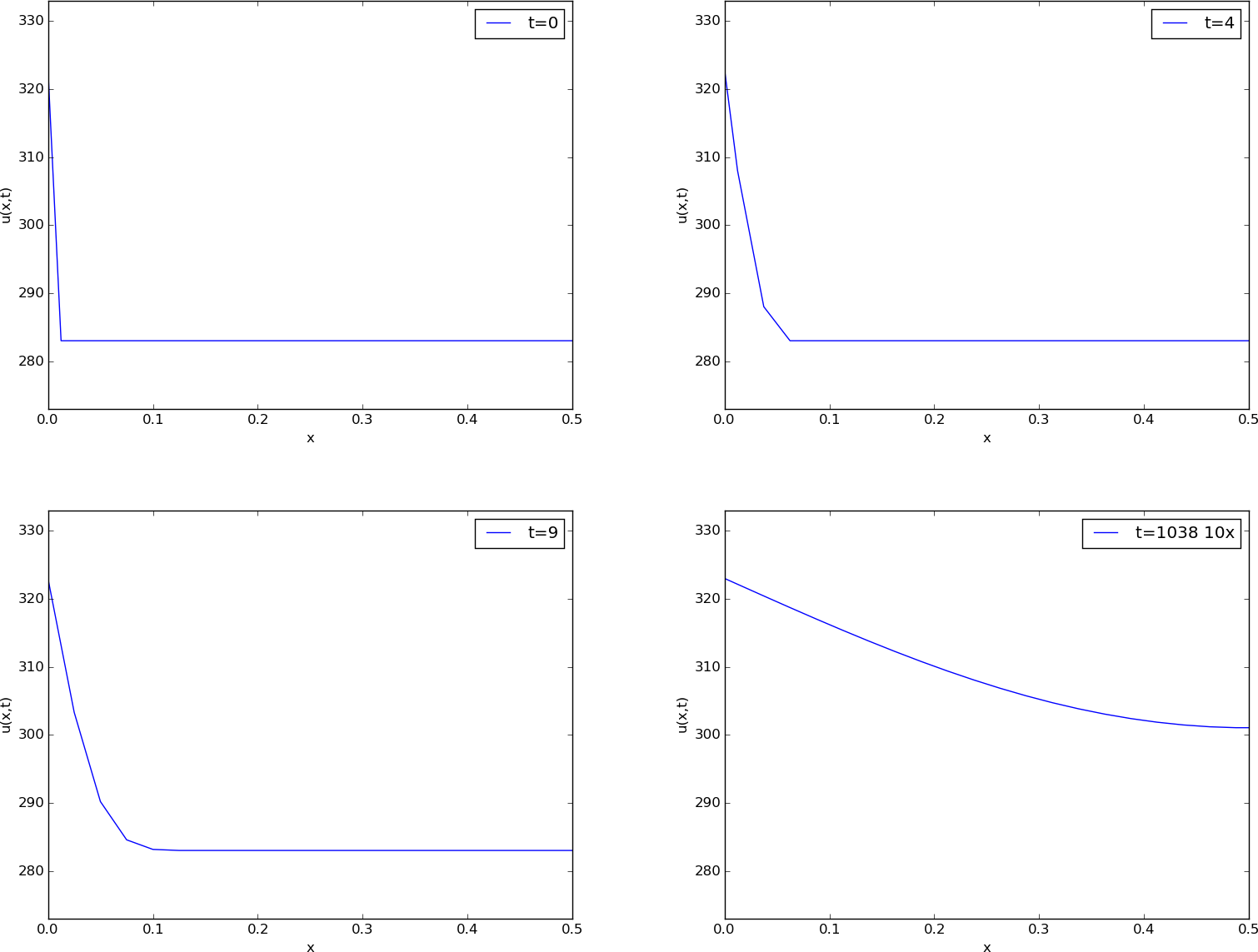
Snapshots of temperature distribution.