Computing integrals

We now turn our attention to solving mathematical problems through computer programming. There are many reasons to choose integration as our first application. Integration is well known already from high school mathematics. Most integrals are not tractable by pen and paper, and a computerized solution approach is both very much simpler and much more powerful - you can essentially treat all integrals $ \int_a^bf(x)dx $ in 10 lines of computer code (!). Integration also demonstrates the difference between exact mathematics by pen and paper and numerical mathematics on a computer. The latter approaches the result of the former without any worries about rounding errors due to finite precision arithmetics in computers (in contrast to differentiation, where such errors prevent us from getting a result as accurate as we desire on the computer). Finally, integration is thought of as a somewhat difficult mathematical concept to grasp, and programming integration should greatly help with the understanding of what integration is and how it works. Not only shall we understand how to use the computer to integrate, but we shall also learn a series of good habits to ensure your computer work is of the highest scientific quality. In particular, we have a strong focus on how to write Matlab code that is free of programming mistakes.

Calculating an integral is traditionally done by $$ \begin{equation} \int_a^b f(x)\,dx = F(b) - F(a), \tag{3.1} \end{equation} $$ where $$ f(x) = \frac{dF}{dx} \thinspace . $$ The major problem with this procedure is that we need to find the anti-derivative $ F(x) $ corresponding to a given $ f(x) $. For some relatively simple integrands $ f(x) $, finding $ F(x) $ is a doable task, but it can very quickly become challenging, even impossible!

The method (3.1) provides an exact or analytical value of the integral. If we relax the requirement of the integral being exact, and instead look for approximate values, produced by numerical methods, integration becomes a very straightforward task for any given $ f(x) $ (!).

The downside of a numerical method is that it can only find an approximate answer. Leaving the exact for the approximate is a mental barrier in the beginning, but remember that most real applications of integration will involve an $ f(x) $ function that contains physical parameters, which are measured with some error. That is, $ f(x) $ is very seldom exact, and then it does not make sense to compute the integral with a smaller error than the one already present in $ f(x) $.

Another advantage of numerical methods is that we can easily integrate a function $ f(x) $ that is only known as samples, i.e., discrete values at some $ x $ points, and not as a continuous function of $ x $ expressed through a formula. This is highly relevant when $ f $ is measured in a physical experiment.

Basic ideas of numerical integration

We consider the integral $$ \begin{equation} \int_a^b f(x)dx\thinspace . \tag{3.2} \end{equation} $$ Most numerical methods for computing this integral split up the original integral into a sum of several integrals, each covering a smaller part of the original integration interval $ [a,b] $. This re-writing of the integral is based on a selection of integration points $ x_i $, $ i = 0,1,\ldots,n $ that are distributed on the interval $ [a,b] $. Integration points may, or may not, be evenly distributed. An even distribution simplifies expressions and is often sufficient, so we will mostly restrict ourselves to that choice. The integration points are then computed as $$ \begin{equation} x_i = a + ih,\quad i = 0,1,\ldots,n, \tag{3.3} \end{equation} $$ where $$ \begin{equation} h = \frac{b-a}{n}\thinspace . \tag{3.4} \end{equation} $$ Given the integration points, the original integral is re-written as a sum of integrals, each integral being computed over the sub-interval between two consecutive integration points. The integral in (3.2) is thus expressed as $$ \begin{equation} \int_a^b f(x)dx = \int_{x_0}^{x_1} f(x)dx + \int_{x_1}^{x_2} f(x)dx + \ldots + \int_{x_{n-1}}^{x_n} f(x)dx\thinspace . \tag{3.5} \end{equation} $$ Note that $ x_0 = a $ and $ x_n = b $.

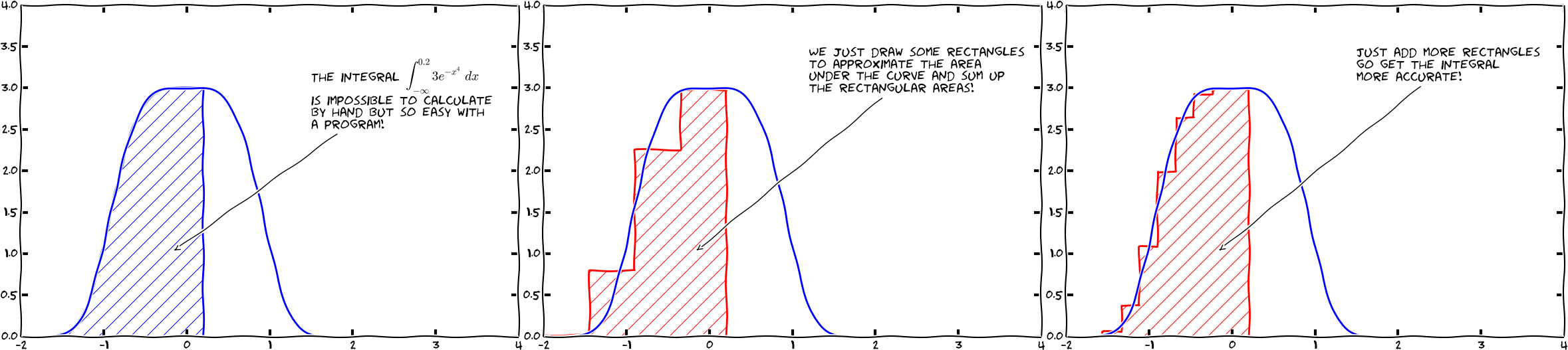
Proceeding from (3.5), the different integration methods will differ in the way they approximate each integral on the right hand side. The fundamental idea is that each term is an integral over a small interval $ [x_i,x_{i+1}] $, and over this small interval, it makes sense to approximate $ f $ by a simple shape, say a constant, a straight line, or a parabola, which we can easily integrate by hand. The details will become clear in the coming examples.

Computational example

To understand and compare the numerical integration methods, it is advantageous to use a specific integral for computations and graphical illustrations. In particular, we want to use an integral that we can calculate by hand such that the accuracy of the approximation methods can easily be assessed. Our specific integral is taken from basic physics. Assume that you speed up your car from rest and wonder how far you go in $ T $ seconds. The distance is given by the integral $ \int_0^T v(t)dt $, where $ v(t) $ is the velocity as a function of time. A rapidly increasing velocity function might be $$ \begin{equation} v\left(t\right) = 3t^{2}e^{t^3}\thinspace . \tag{3.6} \end{equation} $$ The distance after one second is $$ \begin{equation} \int_0^1 v(t)dt, \tag{3.7} \end{equation} $$ which is the integral we aim to compute by numerical methods. Fortunately, the chosen expression of the velocity has a form that makes it easy to calculate the anti-derivative as $$ \begin{equation} V(t) = e^{t^3}-1\thinspace . \tag{3.8} \end{equation} $$ We can therefore compute the exact value of the integral as $ V(1)-V(0)\approx 1.718 $ (rounded to 3 decimals for convenience).