Solving ordinary differential equations
Differential equations constitute one of the most powerful mathematical tools to understand and predict the behavior of dynamical systems in nature, engineering, and society. A dynamical system is some system with some state, usually expressed by a set of variables, that evolves in time. For example, an oscillating pendulum, the spreading of a disease, and the weather are examples of dynamical systems. We can use basic laws of physics, or plain intuition, to express mathematical rules that govern the evolution of the system in time. These rules take the form of differential equations. You are probably well experienced with equations, at least equations like \( ax+b=0 \) or \( ax^2 + bx + c=0 \). Such equations are known as algebraic equations, and the unknown is a number. The unknown in a differential equation is a function, and a differential equation will almost always involve this function and one or more derivatives of the function. For example, \( f'(x)=f(x) \) is a simple differential equation (asking if there is any function \( f \) such that it equals its derivative - you might remember that \( e^x \) is a candidate).
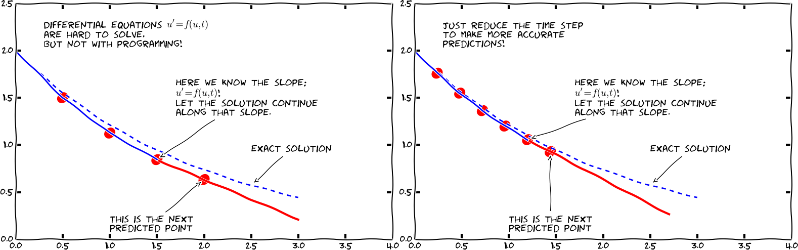
The present chapter starts with explaining how easy it is to solve both single (scalar) first-order ordinary differential equations and systems of first-order differential equations by the Forward Euler method. We demonstrate all the mathematical and programming details through two specific applications: population growth and spreading of diseases.
Then we turn to a physical application: oscillating mechanical systems, which arise in a wide range of engineering situations. The differential equation is now of second order, and the Forward Euler method does not perform well. This observation motivates the need for other solution methods, and we derive the Euler-Cromer scheme , the 2nd- and 4th-order Runge-Kutta schemes, as well as a finite difference scheme (the latter to handle the second-order differential equation directly without reformulating it as a first-order system). The presentation starts with undamped free oscillations and then treats general oscillatory systems with possibly nonlinear damping, nonlinear spring forces, and arbitrary external excitation. Besides developing programs from scratch, we also demonstrate how to access ready-made implementations of more advanced differential equation solvers in Matlab.
3: The term scheme is used as synonym for method or computational recipe, especially in the context of numerical methods for differential equations.
As we progress with more advanced methods, we develop more sophisticated and reusable programs, and in particular, we incorporate good testing strategies so that we bring solid evidence to correct computations. Consequently, the beginning with population growth and disease modeling examples has a very gentle learning curve, while that curve gets significantly steeper towards the end of the treatment of differential equations for oscillatory systems.