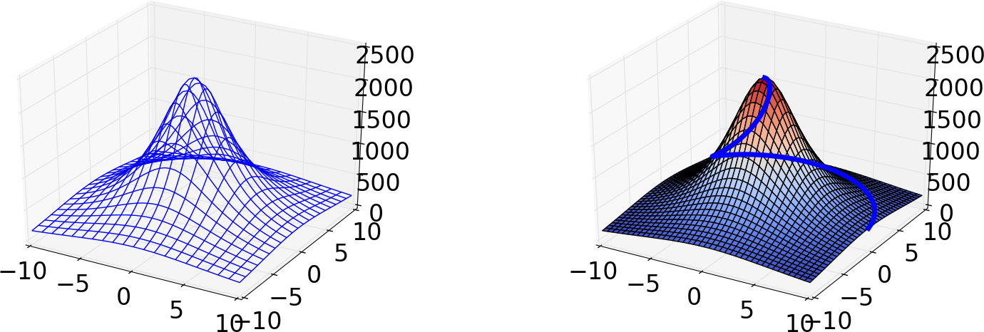
Figure 12: Two different plots of a mountain. The right plot also shows a trajectory to the top of the mountain.
This chapter is taken from the book A Primer on Scientific Programming with Python by H. P. Langtangen, 5th edition, Springer, 2016.
Vectors appeared when mathematicians needed to calculate with a list of numbers. When they needed a table (or a list of lists in Python terminology), they invented the concept of matrix (singular) and matrices (plural). A table of numbers has the numbers ordered into rows and columns. One example is $$ \begin{equation*} \left\lbrack\begin{array}{cccc} 0 & 12 & -1 & 5\\ -1 & -1 & -1 & 0\\ 11 & 5 & 5 & -2 \end{array}\right\rbrack \end{equation*} $$ This table with three rows and four columns is called a \( 3\times4 \) matrix (mathematicians may not like this sentence, but it suffices for our purposes). If the symbol \( A \) is associated with this matrix, \( A_{i,j} \) denotes the number in row number \( i \) and column number \( j \). Counting rows and columns from 0, we have, for instance, \( A_{0,0}=0 \) and \( A_{2,3}=-2 \). We can write a general \( m\times n \) matrix \( A \) as $$ \begin{equation*} \left\lbrack\begin{array}{ccc} A_{0,0} & \cdots & A_{0,n-1}\\ \vdots & \ddots & \vdots\\ A_{m-1,0} & \cdots & A_{m-1,n-1} \end{array}\right\rbrack \end{equation*} $$ Matrices can be added and subtracted. They can also be multiplied by a scalar (a number), and there is a concept of length or size. The formulas are quite similar to those presented for vectors, but the exact form is not important here.
We can generalize the concept of table and matrix to array, which holds quantities with in general \( d \) indices. Equivalently we say that the array has rank \( d \). For \( d=3 \), an array \( A \) has elements with three indices: \( A_{p,q,r} \). If \( p \) goes from 0 to \( n_p-1 \), \( q \) from 0 to \( n_q-1 \), and \( r \) from 0 to \( n_r-1 \), the \( A \) array has \( n_p\times n_q\times n_r \) elements in total. We may speak about the shape of the array, which is a \( d \)-vector holding the number of elements in each "array direction", i.e., the number of elements for each index. For the mentioned \( A \) array, the shape is \( (n_p,n_q,n_r) \).
The special case of \( d=1 \) is a vector, and \( d=2 \) corresponds to a matrix. When we program we may skip thinking about vectors and matrices (if you are not so familiar with these concepts from a mathematical point of view) and instead just work with arrays. The number of indices corresponds to what is convenient in the programming problem we try to solve.
Consider a nested list table of two-pairs [C, F]
constructed by
>>> Cdegrees = [-30 + i*10 for i in range(3)]
>>> Fdegrees = [9./5*C + 32 for C in Cdegrees]
>>> table = [[C, F] for C, F in zip(Cdegrees, Fdegrees)]
>>> print table
[[-30, -22.0], [-20, -4.0], [-10, 14.0]]
>>> table2 = np.array(table)
>>> print table2
[[-30. -22.]
 [-20.  -4.]
 [-10.  14.]]
>>> type(table2)
<type 'numpy.ndarray'>
table2 is a two-dimensional array, or an array
of rank 2.
The table list and the table2 array are stored very differently in
memory. The table variable refers to a list object containing three
elements. Each of these elements is a reference to a separate list
object with two elements, where each element refers to a separate
float object. The table2 variable is a reference to a single
array object that again refers to a consecutive sequence of bytes in
memory where the six floating-point numbers are stored. The data
associated with table2 are found in one chunk in the computer's
memory, while the data associated with table are scattered around in
memory. On today's machines, it is much more expensive to find data in
memory than to compute with the data. Arrays make the data fetching
more efficient, and this is major reason for using arrays. However,
this efficiency gain is only present for very large arrays, not for a
\( 3\times 2 \) array.
Indexing a nested list is done in two steps, first the outer list is indexed, giving access to an element that is another list, and then this latter list is indexed:
>>> table[1][0]     # table[1] is [-20,4], whose index 0 holds -20
-20
>>> table2[1][0]
-20.0
>>> table2[1,0]
-20.0
A two-dimensional array reflects a table and has a certain number of
rows and columns. We refer to rows as the first dimension of the
array and columns as the second dimension. These two dimensions are
available as table2.shape:
>>> table2.shape
(3, 2)
A loop over all the elements in a two-dimensional array is usually
expressed as two nested for loops, one for each index:
>>> for i in range(table2.shape[0]):
...     for j in range(table2.shape[1]):
...         print 'table2[%d,%d] = %g' % (i, j, table2[i,j])
...
table2[0,0] = -30
table2[0,1] = -22
table2[1,0] = -20
table2[1,1] = -4
table2[2,0] = -10
table2[2,1] = 14
for loop:
>>> for index_tuple, value in np.ndenumerate(table2):
...     print 'index %s has value %g' % \
...           (index_tuple, table2[index_tuple])
...
index (0,0) has value -30
index (0,1) has value -22
index (1,0) has value -20
index (1,1) has value -4
index (2,0) has value -10
index (2,1) has value 14
In the same way as we can extract sublists of lists, we can extract subarrays of arrays using slices.
table2[0:table2.shape[0], 1]  # 2nd column (index 1)
array([-22.,  -4.,  14.])

>>> table2[0:, 1]             # same
array([-22.,  -4.,  14.])

>>> table2[:, 1]              # same
array([-22.,  -4.,  14.])
>>> t = np.linspace(1, 30, 30).reshape(5, 6)
>>> t
array([[  1.,   2.,   3.,   4.,   5.,   6.],
       [  7.,   8.,   9.,  10.,  11.,  12.],
       [ 13.,  14.,  15.,  16.,  17.,  18.],
       [ 19.,  20.,  21.,  22.,  23.,  24.],
       [ 25.,  26.,  27.,  28.,  29.,  30.]])

>>> t[1:-1:2, 2:]
array([[  9.,  10.,  11.,  12.],
       [ 21.,  22.,  23.,  24.]])
t array and pick out
the two rows corresponding to the first slice 1:-1:2,
       [  7.,   8.,   9.,  10.,  11.,  12.]
       [ 19.,  20.,  21.,  22.,  23.,  24.]
2:,
       [  9.,  10.,  11.,  12.]
       [ 21.,  22.,  23.,  24.]
Another example is
>>> t[:-2, :-1:2]
array([[  1.,   3.,   5.],
       [  7.,   9.,  11.],
       [ 13.,  15.,  17.]])
t that consists of the rows with indices 0 and 3 and the
columns with indices 1 and 2:
>>> t[np.ix_([0,3], [1,2])]
array([[  2.,   3.],
       [ 20.,  21.]])
>>> t[np.ix_([0,3], [1,2])] = 0
>>> t
array([[  1.,   0.,   0.,   4.,   5.,   6.],
       [  7.,   8.,   9.,  10.,  11.,  12.],
       [ 13.,  14.,  15.,  16.,  17.,  18.],
       [ 19.,   0.,   0.,  22.,  23.,  24.],
       [ 25.,  26.,  27.,  28.,  29.,  30.]])
Recall that slices only gives a view to the array, not a copy of the values:
>>> a = t[1:-1:2, 1:-1]
>>> a
array([[  8.,   9.,  10.,  11.],
       [  0.,   0.,  22.,  23.]])
>>> a[:,:] = -99
>>> a
array([[-99., -99., -99., -99.],
       [-99., -99., -99., -99.]])
>>> t  # is t changed to? yes!
array([[  1.,   0.,   0.,   4.,   5.,   6.],
       [  7., -99., -99., -99., -99.,  12.],
       [ 13.,  14.,  15.,  16.,  17.,  18.],
       [ 19., -99., -99., -99., -99.,  24.],
       [ 25.,  26.,  27.,  28.,  29.,  30.]])
The operations on vectors in the section Vector arithmetics and vector functions can quite straightforwardly be extended to arrays of any dimension. Consider the definition of applying a function \( f(v) \) to a vector \( v \): we apply the function to each element \( v_i \) in \( v \). For a two-dimensional array \( A \) with elements \( A_{i,j} \), \( i=0,\ldots,m \), \( j=0,\ldots,n \), the same definition yields $$ \begin{equation*} f(A) = (f(A_{0,0}),\ldots,f(A_{m-1,0}),f(A_{1,0}), \ldots,f(A_{m-1,n-1}))\tp \end{equation*} $$ For an array \( B \) with any rank, \( f(B) \) means applying \( f \) to each array entry.
The asterisk operation from the section Vector arithmetics and vector functions is also naturally extended to arrays: \( A*B \) means multiplying an element in \( A \) by the corresponding element in \( B \), i.e., element \( (i,j) \) in \( A*B \) is \( A_{i,j}B_{i,j} \). This definition naturally extends to arrays of any rank, provided the two arrays have the same shape.
Adding a scalar to an array implies adding the scalar to each element in the array. Compound expressions involving arrays, e.g., \( \exp(-A^2)*A +1 \), work as for vectors. One can in fact just imagine that all the array elements are stored after each other in a long vector (this is actually the way the array elements are stored in the computer's memory), and the array operations can then easily be defined in terms of the vector operations from the section Vector arithmetics and vector functions.
Readers with knowledge of matrix computations may get confused by the
meaning of \( A^2 \) in matrix computing and \( A^2 \) in array computing. The
former is a matrix-matrix product, while the latter means squaring all
elements of \( A \). Which rule to apply, depends on the context, i.e.,
whether we are doing linear algebra or vectorized arithmetics. In
mathematical typesetting, \( A^2 \) can be written as \( AA \), while the
array computing expression \( A^2 \) can be alternatively written as
\( A*A \). In a program, A*A and A**2 are identical computations,
meaning squaring all elements (array arithmetics). With NumPy arrays
the matrix-matrix product is obtained by dot(A, A). The
matrix-vector product \( Ax \), where \( x \) is a vector, is computed by
dot(A, x). However, with matrix objects (see the section Matrix objects) A*A implies the mathematical matrix
multiplication \( AA \).
This section only makes sense if you are familiar with basic linear
algebra and the matrix concept. The arrays created so far have been
of type ndarray. NumPy also has a matrix type called matrix or
mat for one- and two-dimensional arrays. One-dimensional arrays are
then extended with one extra dimension such that they become matrices,
i.e., either a row vector or a column vector:
>>> import numpy as np
>>> x1 = np.array([1, 2, 3], float)
>>> x2 = np.matrix(x1)          # or mat(x1)
>>> x2                          # row vector
matrix([[ 1.,  2.,  3.]])
>>> x3 = mat(x1).T              # transpose = column vector
>>> x3
matrix([[ 1.],
        [ 2.],
        [ 3.]])

>>> type(x3)
<class 'numpy.matrixlib.defmatrix.matrix'>
>>> isinstance(x3, np.matrix)
True
matrix objects is that the multiplication
operator represents the matrix-matrix, vector-matrix, or matrix-vector
product as we know from linear algebra:
>>> A = np.eye(3)                 # identity matrix
>>> A
array([[ 1.,  0.,  0.],
       [ 0.,  1.,  0.],
       [ 0.,  0.,  1.]])
>>> A = mat(A)
>>> A
matrix([[ 1.,  0.,  0.],
        [ 0.,  1.,  0.],
        [ 0.,  0.,  1.]])
>>> y2 = x2*A                     # vector-matrix product
>>> y2
matrix([[ 1.,  2.,  3.]])
>>> y3 = A*x3                     # matrix-vector product
>>> y3
matrix([[ 1.],
        [ 2.],
        [ 3.]])
ndarray objects is quite different!
Readers who are familiar with MATLAB, or intend to use Python and
MATLAB together, should seriously think about programming with
matrix objects instead of ndarray objects, because the matrix
type behaves quite similar to matrices and vectors in MATLAB.
Nevertheless, matrix cannot be used for arrays of larger dimension
than two.
Python has strong support for numerical linear algebra, much like the functionality found in MATLAB. Some of the most widely used operations are exemplified below.
We start with showing how to find the inverse and the determinant of a matrix, and how to compute the eigenvalues and eigenvectors:
>>> import numpy as np
>>> A = np.array([[2, 0], [0, 5]], dtype=float)

>>> np.linalg.inv(A)  # inverse matrix
array([[ 0.5,  0. ],
       [ 0. ,  0.2]])

>>> np.linalg.det(A)  # determinant
9.9999999999999982

>>> eig_values, eig_vectors = np.linalg.eig(A)
>>> eig_values
array([ 2.,  5.])
>>> eig_vectors
array([[ 1.,  0.],
       [ 0.,  1.]])
The np.dot function is used for scalar or dot product as well as
matrix-vector and matrix-matrix products between array objects:
>>> a = np.array([4, 0])
>>> b = np.array([0, 1])
>>> np.dot(A, a)         # matrix vector product
array([ 8.,  0.])
>>> np.dot(a, b)         # dot product between vectors
0
>>>
>>> B = np.ones((2, 2))  # 2x2 matrix with 1's
>>> np.dot(A, B)         # matrix-matrix product
array([[ 2.,  2.],
       [ 5.,  5.]])
Note that using the matrix class instead of plain arrays
(see the section Matrix objects)
allows * to be used as operator for matrix-vector and matrix-matrix
products.
The cross product \( a\times b \), between vectors \( a \) and \( b \) of length 3, is computed by
>>> np.cross([1, 1, 1], [0, 0, 1])
array([ 1, -1,  0])
>>> np.arccos(np.dot(a, b)/(np.linalg.norm(a)*np.linalg.norm(b)))
1.5707963267948966
Various norms of matrices and vectors are well supported by NumPy. Some common examples are
>>> np.linalg.norm(A)        # Frobenius norm for matrices
5.3851648071345037
>>> np.sqrt(np.sum(A**2))    # Frobenius norm: direct formula
5.3851648071345037
>>> np.linalg.norm(a)        # l2 norm for vectors
4.0
pydoc numpy.linalg.norm for information on other norms.
The sum of all elements or of the elements in a particular row or column
is computed by np.sum:
>>> np.sum(B)          # sum of all elements
2.0
>>> B.sum()            # sum of all elements; alternative syntax
2.0
>>> np.sum(B, axis=0)  # sum over index 0 (rows)
array([ 4., -2.])
>>> np.sum(B, axis=1)  # sum over index 1 (columns)
array([ 3., -1.])
>>> np.max(B)          # max over all elements
3.0
>>> B.max()            # max over all elements, alt. syntax
3.0
>>> np.min(B)          # min over all elements
-4.0
>>> np.abs(B).min()    # min absolute value
1.0
>>> I = np.eye(2)   # identity matrix of size 2
>>> I
array([[ 1.,  0.],
       [ 0.,  1.]])
>>> np.abs(np.dot(A, np.linalg.inv(A)) - I).max()
0.0
== when testing real numbers!
It could be tempting to test \( AA^{-1}=I \) using the syntax
>>> np.dot(A, np.linalg.inv(A)) == np.eye(2)
array([[ True,  True],
       [ True,  True]], dtype=bool)
if test== for matrices with float elements may fail because of
rounding errors== fails:
>>> A = np.array([[4, 0], [0, 49]], dtype=float)
>>> np.dot(A, np.linalg.inv(A)) == np.eye(2)
array([[ True,  True],
       [ True, False]], dtype=bool)
1.0/49*49 is not exactly 1 because of rounding errors.)
The first problem is solved by using the C.all(), which returns one
boolean variable True if all elements in the boolean array C are True,
otherwise it returns False, as in the case above:
>>> (np.dot(A, np.linalg.inv(A)) == np.eye(2)).all()
False
Indexing an element is done by A[i,j]. A row or column
is extracted as
>>> A[0,:]  # first row
array([ 2.,  0.])
>>> A[:,1]  # second column
array([ 0.,  5.])
np.ix_
function. Here is an example where we
grab row 0 and 2, then column 1:
>>> C = np.array([[1,2,3],[4,5,6],[7,8,9]])
>>> C[np.ix_([0,2], [1])]  # row 0 and 2, then column 1
array([[2],
       [8]])
You can also use the colon notation to pick out other parts of a matrix.
If C is a \( 3\times 5 \)-matrix,
C[1:3, 0:4]
C after the first, and the first four columns of C (recall that the upper limits, here 3 and 4, are
not included).
Readers familiar with MATLAB should note that the indexing may
be a bit unexpected when referring to parts of a matrix: writing
C[[0, 2], [0, 2]] one would expect entries residing in rows/columns
\( 0 \) and \( 2 \), but that behavior requires in Python the np.ix_
command:
>>> C = np.array([[1, 2, 3], [4, 5, 6], [7, 8, 9]])
>>> C[np.ix_([0, 2], [0, 2])]
[[1 3]
 [7 9]]
>>> # Grab row 0, 2, then column 0 from row 0 and column 2 from row 2
>>> C[[0, 2], [0, 2]]
[1 9]
The transpose of a matrix B is obtained by B.T:
>>> B = np.array([[1, 2], [3, -4]], dtype=float)
>>> B.T                # the transpose
array([[ 1.,  3.],
       [ 2., -4.]])
NumPy has rich functionality for doing operations on array objects. For example, one can strip down a matrix to its upper or lower triangular parts:
>>> np.triu(B)  # upper triangular part of B
array([[ 1.,  2.],
       [ 0., -4.]])
>>> np.tril(B)  # lower triangular part of B
array([[ 1.,  0.],
       [ 3., -4.]])
The perhaps most frequent operation in linear algebra is the solution
of systems of linear algebraic equations: \( Ax=b \), where \( A \) is a coefficient
matrix, \( b \) is a given right-hand side vector, and \( x \) is the solution vector.
The function np.linalg.solve(A, b) does the job:
>>> A = np.array([[1, 2], [-2, 2.5]])
>>> x = np.array([-1, 1], dtype=float)  # pick a solution
>>> b = np.dot(A, x)                    # find right-hand side

>>> np.linalg.solve(A, b)               # will this compute x?
array([-1.,  1.])
Implementing Gaussian elimination constitutes a good pedagogical example on how to perform row and column operations on a matrix. Some needed functionality is
A[[i, j]] = A[[j, i]]  # swap rows i and j
A[i] *= k              # multiply row i by a constant k
A[j] += k*A[i]         # add row i, multiplied by k, to row j
m, n = shape(A)
for j in range(n - 1):
    for i in range(j + 1, m):
        A[i,j:] -= (A[i,j]/A[j,j])*A[j,j:]
j:, which refers to indices from j and up to the end of the array.
More generally, when referring to an array a with length n, the following are equivalent:
a[0:n]
a[:n]
a[0:]
a[:]
A[j,j] become zero along the way. To avoid
this, we can swap rows when the problem arises. The following code
implements the idea and will not fail, even if some of the columns are zero.
def Gaussian_elimination(A):
    rank = 0
    m, n = np.shape(A)
    i = 0
    for j in range(n):
        p = np.argmax(abs(A[i:m,j]))
        if p > 0: # swap rows
            A[[i,p+i]] = A[[p+i, i]]
        if A[i,j] != 0:
            # j is a pivot column
            rank += 1
            for r in range(i+1, m):
                A[r,j:] -= (A[r,j]/A[i,j])*A[i,j:]
            i += 1
        if i > m:
            break
    return A, rank
A and its rank.
The rank of a matrix equals the number of pivot columns after Gaussian
elimination. The variable rank counts these in the code above.
Due to rounding errors, the computed rank may be higher than the
actual rank: the rounding errors may imply that A[i,j] != 0 is true,
even if Gaussian elimination performed in exact arithmetics gives exactly zero.
Such situations can be avoided by replacing if A[i,j] !=0:
with if abs(A[i,j]) > tol:, where tol is some small
tolerance.
A more reliable way to compute the rank is to compute the
singular value decomposition of A, and check how many of the
singular values that are larger than a threshold epsilon:
>>> A = np.array([[1, 2.01], [2.01, 4.0401]])
>>> U, s, V = np.linalg.svd(A) # s are the singular values of A
# abs(s) > tol gives an array with True and False values
# s.nonzero() lists indices k so that s[k] != 0
>>> shape((abs(s) > tol).nonzero())[1]  # rank
1
>>> A, rank = Gaussian_elimination(A)
>>> rank
2
if abs(A[i,j]) > 1E-10:
in the function Gaussian_elimination, the code will say that the rank is 1,
which is the correct value also found by using the singular value
decomposition.
It is known that the determinant is nonzero if and only if the rank equals the number of rows/columns. For the matrix \( A \) we used above, the determinant should thus be \( 0 \), but also here roundoff errors come into play:
>>> A = np.array([[1, 2.01], [2.01, 4.0401]])
>>> A[0, 0]*A[1, 1] - A[0, 1]*A[1, 0]
8.881784197e-16
>>> np.linalg.det(A)
8.92619311799e-16
Using our own Gaussian elimination function for computing the rank is less efficient than calling NumPy's singular value decomposition. Here are timings for a random \( 100\times 100 \)-matrix:
>>> A = np.random.uniform(0, 1, (100, 100))
>>> %timeit U, s, V = np.linalg.svd(A)
100 loops, best of 3: 3.7 ms per loop
>>> %timeit A, rank = Gaussian_elimination(A)
100 loops, best of 3: 22.3 ms per loop
SymPy supports symbolic computations also for linear algebra operations. We may create a matrix and find its inverse and determinant:
>>> import sympy as sym
>>> A = sym.Matrix([[2, 0], [0, 5]])

>>> A**-1    # the inverse
Matrix([
[1/2,   0],
[  0, 1/5]])

>>> A.inv()  # the inverse
Matrix([
[1/2,   0],
[  0, 1/5]])

>>> A.det()  # the determinant
10
sym.Rational objects to be precise).
Eigenvalues can also be computed exactly:
>>> A.eigenvals()
{2: 1, 5: 1}
>>> e = list(A.eigenvals().keys())
>>> e
[2, 5]
>>> A.eigenvects()
[(2, 1, [Matrix([
[1],
[0]])]), (5, 1, [Matrix([
[0],
[1]])])]
sym.Matrix object.
To isolate the first eigenvector, we can index the list and tuple:
>>> v1 = A.eigenvects()[0][2]
>>> v1
Matrix([
[1],
[0]])
sym.Matrix object with two indices. To extract the
vector elements in a plain list, we can do this:
>>> v1 = [v1[i,0] for i in range(v1.shape[0])]
>>> v1
[1, 0]
>>> v = [[t[2][0][i,0] for i in range(t[2][0].shape[0])]
         for t in A.eigenvects()]
>>> v
[[1, 0], [0, 1]]
The norm of a matrix or vector is an exact expression:
>>> A.norm()
sqrt(29)
>>> a = sym.Matrix([1, 2])   # vector [1, 2]
>>> a
Matrix([
[1],
[2]])
>>> a.norm()
sqrt(5)
The matrix-vector product and the dot product between vectors are done like this:
>>> A*a                      # matrix*vector
Matrix([
[ 2],
[10]])
>>> b = sym.Matrix([2, -1])  # vector [2, -1]
>>> a.dot(b)
0
Solving linear systems exactly is also possible:
>>> x = sym.Matrix([-1, 1])/2
>>> x
Matrix([
[-1/2],
[ 1/2]])
>>> b = A*x
>>> x = A.LUsolve(b)  # does it compute x?
>>> x                 # x is a matrix object
Matrix([
[-1/2],
[ 1/2]])
x to a plain numpy array with
float values:
>>> x = np.array([float(x[i,0].evalf())
                  for i in range(x.shape[0])])
>>> x
array([-0.5,  0.5])
Exact row operations can be done as exemplified here:
>>> A[1,:] + 2*A[0,:]  # [0,5] + 2*[2,0]
Matrix([[4, 5]])
Visualization of scalar and vector fields in Python is commonly done using Matplotlib or Mayavi. Both packages support basic visualization of 2D scalar and vector fields, but Mayavi offers more advanced three-dimensional visualization techniques, especially for 3D scalar and vector fields.
One can also use SciTools for visualizing 2D scalar and vector fields, using either Matplotlib, Gnuplot, or VTK as plotting engines, but this topic is omitted from the present book. However, for fast visualization of large 2D scalar fields, Gnuplot is a viable tool, and the SciTools interface offers a convenient MATLAB-style set of commands to operate Gnuplot.
To exemplify visualization of scalar and vector fields with Matplotlib and Mayavi, we use a common set of examples. A scalar function of \( x \) and \( y \) is visualized either as a flat two-dimensional plot with contour lines of the field, or as a three-dimensional surface where the height of the surface corresponds to the function value of the field. In the latter case we also add a three-dimensional parameterized curve to the plot.
To illustrate plotting of vector fields, we simply plot the gradient of the scalar field, together with the scalar field. Our convention for variable names goes as follows:
x, y for one-dimensional coordinates along each axis direction.xv, yv for the corresponding
vectorized coordinates in a 2D.u, v for the components of a vector field
at points corresponding to xv, yv.Previously in the book we have explained how to obtain Matplotlib for various platforms. To obtain Mayavi on Ubuntu platforms you can write
pip install mayavi --upgrade
conda install mayavi
We consider the 2D scalar field defined by $$ \begin{equation} h(x,y) = \frac{h_0}{1+ \frac{x^2+y^2}{R^2}}. \tag{13} \end{equation} $$ \( h(x,y) \) may model the height of an isolated circular mountain, \( h \) being the height above sea level, while \( x \) and \( y \) are Cartesian coordinates on the earth's surface, \( h_0 \) the height of the mountain, and \( R \) the radius of the mountain. Since mountains are actually quite flat (or more precisely, their heights are small compared to the horizontal extent), we use meter as length unit for vertical distances (\( z \) direction) and km as length unit for horizontal distances (\( x \) and \( y \) coordinates). Prior to all code below we have initialized \( h_0 \) and \( R \) with the following values: \( h_0=2277 \) m and \( R=4 \) km.
Before we can plot \( h(x,y) \), we need to create a rectangular grid in the \( xy \) plane with all the points used for plotting. Regardless of which plotting package we will use later on, the grid can be made as follows:
x = y = np.linspace(-10., 10., 41)
xv, yv = np.meshgrid(x, y, indexing='ij', sparse=False)

hv = h0/(1 + (xv**2+yv**2)/(R**2))
x and y in the
interval \( [-10,10] \) km.
Note the mysterious extra parameters to meshgrid here, which are needed in order for the coordinates to have the right order such that the arithmetics
in the expression for hv becomes correct.
The expression computes the
surface value at the \( 41\times 41 \) grid points in one vectorized operation.
A surface plot of a 2D scalar field \( h(x,y) \) is a visualization of the surface \( z=h(x,y) \) in three-dimensional space. Most plotting packages have functions which can be used to create surface plots of 2D scalar fields. These can be either wireframe plots, where only lines connecting the grid points are drawn, or plots where the faces of the surface are colored. In Figure 12 we have shown two such plots of the surface \( h(x,y) \). The section Surface plots presents the code which generates these plots.
Figure 12: Two different plots of a mountain. The right plot also shows a trajectory to the top of the mountain.
To illustrate the plotting of three-dimensional parameterized curves, we consider a trajectory that represents a circular climb to the top of the mountain: $$ \begin{align} \boldsymbol{r}(t) = & \left( 10\left(1 - \frac{t}{2\pi}\right)\cos(t) \right) \boldsymbol{i} + \left( 10\left(1 - \frac{t}{2\pi}\right)\sin(t) \right) \boldsymbol{j} \nonumber\\ & + \frac{h_0}{1 + \frac{100(1 - t/(2\pi))^2}{R^2}} \boldsymbol{k}. \tag{14} \end{align} $$ Here \( \boldsymbol{i} \), \( \boldsymbol{j} \), and \( \boldsymbol{k} \) denote the unit vectors in the \( x \)-, \( y \)-, and \( z \)-directions, respectively. The coordinates of \( \boldsymbol{r}(t) \) can be produced by
s = np.linspace(0, 2*np.pi, 100)
curve_x = 10*(1 - s/(2*np.pi))*np.cos(s)
curve_y = 10*(1 - s/(2*np.pi))*np.sin(s)
curve_z = h0/(1 + 100*(1 - s/(2*np.pi))**2/(R**2))
Contour lines are lines defined by the implicit equation \( h(x,y)=C \), where \( C \) is some constant representing the contour level. Normally, we let \( C \) run over some equally spaced values, and very often, the plotting program computes the \( C \) values. To distinguish contours, one often associates each contour level \( C \) with its own color.
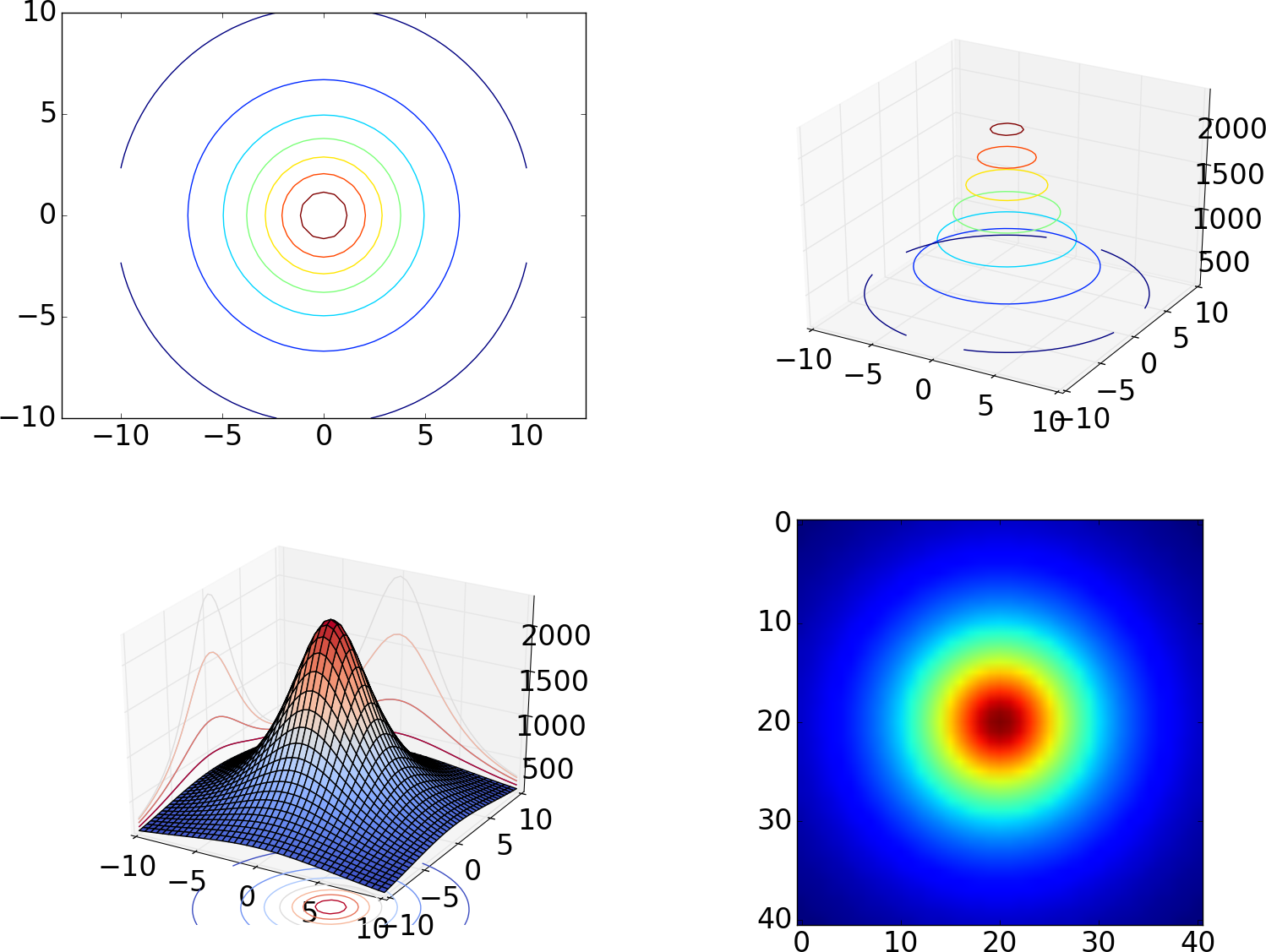
Figure 13 shows different ways contour lines can be used to visualize the surface \( h(x,y) \). The first and last plot are visualizations utilizing two spatial dimensions. The first draws a small set of contour lines only, while the last one displays the surface as an image, whose colors reflect the values of the field, or equivalently, the height of the surface. The third plot actually combines three different types of contours, each type corresponding to keeping a coordinate constant and projecting the contours on a "wall". The code used to generate these plots is presented in the section Contour plots.
Figure 13: Different types of contour plots of a 2D scalar field in two and three dimensions.
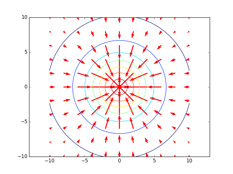
The gradient vector field \( \nabla h \) of a 2D scalar field \( h(x,y) \) is defined by $$ \begin{equation} \nabla h = \frac{\partial h}{\partial x}\boldsymbol{i} + \frac{\partial h}{\partial y}\boldsymbol{j}. \tag{15} \end{equation} $$ One learns in vector calculus that the gradient points in the direction where \( h \) increases most, and that the gradients are orthogonal to the contour lines. This is something we can easily illustrate by creating 2D plots of the contours and the gradient field. A challenge in making such plots is to get the right arrow lengths so that the arrows are well visible, but they do not collide and make a cluttered visual impression. Since the arrows are drawn at each point in a 2D grid, one way of controlling the number of arrows is to control the resolution of the grid.
So, let us create a grid with 20 instead of 40 intervals in the horizontal directions:
x2 = y2 = np.linspace(-10.,10.,11)
x2v, y2v = np.meshgrid(x2, y2, indexing='ij', sparse=False)
h2v = h0/(1 + (x2v**2 + y2v**2)/(R**2)) # h on coarse grid
np.gradient:
dhdx, dhdy = np.gradient(h2v) # dh/dx, dh/dy
Figure 14: Gradient field with contour plot.
We import any visualization package under the name plt, so
for Matplotlib the import is done by
import matplotlib.pyplot as plt
Axes object, named ax and made by
fig = plt.figure(1)   # Get current figure
ax = fig.gca()        # Get current axes
from mpl_toolkits.mplot3d import Axes3D

fig = plt.figure(1)
ax = fig.gca(projection='3d')
The Matplotlib functions for producing surface plots of 2D scalar fields are
ax.plot_wireframe and ax.plot_surface.
The first one produces a wireframe plot, and the second one colors the surface.
The following code uses the functions to produce the plots shown in Figure
12, once the grid has been defined as in the section Surface plots,
and the coordinates of the parameterized curve have been computed as in the section Parameterized curve.
fig = plt.figure(1)
ax = fig.gca(projection='3d')
ax.plot_wireframe(xv, yv, hv, rstride=2, cstride=2)

# Simple plot of mountain and parametric curve
fig = plt.figure(2)
ax = fig.gca(projection='3d')
from matplotlib import cm
ax.plot_surface(xv, yv, hv, cmap=cm.coolwarm,
                rstride=1, cstride=1)

# add the parametric curve. linewidth controls the width of the curve
ax.plot(curve_x, curve_y, curve_z, linewidth=5)
plt.show() command is necessary to force Matplotlib to show a plot on the screen.
Note that the second plot in this figure is drawn using a finer grid.
This is controlled with the rstride and cstride parameters, which
sets the number of grid lines in each direction. Setting one of these
to 1 means that a grid line is drawn for every value in the grid in
the corresponding direction, and setting to 2 means that a grid line
will be drawn for every two values in the grid. You will normally need
to experiment with such parameters to get a visually attractive plot.
A surface with colors reflecting the height of the surface
needs specification of a color map, which is
a mapping between function values and colors.
Above we applied the common coolwarm
scheme which goes from blue ("cool" color for minimum values) to red
("warm" color for maximum values).
There are lots of colormaps to choose from, and you have
to experiment to find appropriate choices according to your taste and
to the problem at hand.
To the latter plot we also added the parameterized curve \( \boldsymbol{r}(t) \),
defined by (14), using the command plot. The
attribute linewidth is increased here in order to make the curve thicker and
more visible. By default, Matplotlib adds plots to each other without
any need for plt.hold('on'), although such a command can indeed be
used.
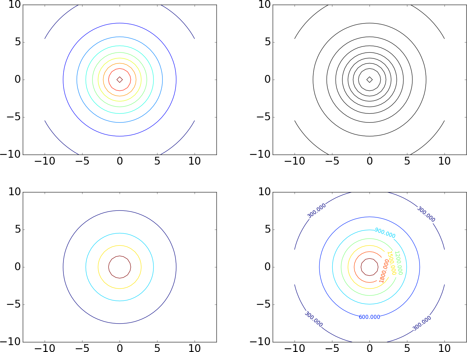
The following code exemplifies different types of contour plots. The first two plots (default two-dimensional and three-dimensional contour plots) are shown in Figure 13. The next four plots appear in Figure 15. Note that, when we asked Matplotlib to plot 10 contours, the response was, surprisingly, 9 contour lines, where one of the contours was incomplete. This kind of behavior may also be found in other plotting packages (such as MATLAB): the package will do its best to plot the requested number of complete contour lines, but there is no guarantee that this number is achieved exactly.
# Default two-dimensional contour plot with 7 colored lines
fig = plt.figure(3)
ax = fig.gca()
ax.contour(xv, yv, hv)
plt.axis('equal')

# Default three-dimensional contour plot
fig = plt.figure(4)
ax = fig.gca(projection='3d')
ax.contour(xv, yv, hv)

# Plot of mountain and contour lines projected on the
# coordinate planes
fig = plt.figure(5)
ax = fig.gca(projection='3d')
ax.plot_surface(xv, yv, hv, cmap=cm.coolwarm,
                rstride=1, cstride=1)
# zdir is the projection axis
# offset is the offset of the projection plane
ax.contour(xv, yv, hv, zdir='z', offset=-1000, cmap=cm.coolwarm)
ax.contour(xv, yv, hv, zdir='x', offset=-10,   cmap=cm.coolwarm)
ax.contour(xv, yv, hv, zdir='y', offset=10,    cmap=cm.coolwarm)

# View the contours by displaying as an image
fig = plt.figure(6)
ax = fig.gca()
ax.imshow(hv)

# 10 contour lines (equally spaced contour levels)
fig = plt.figure(7)
ax = fig.gca()
ax.contour(xv, yv, hv, 10)
plt.axis('equal')

# 10 black ('k') contour lines
fig = plt.figure(8)
ax = fig.gca()
ax.contour(xv, yv, hv, 10, colors='k')
plt.axis('equal')

# Specify the contour levels explicitly as a list
fig = plt.figure(9)
ax = fig.gca()
levels = [500., 1000., 1500., 2000.]
ax.contour(xv, yv, hv, levels=levels)
plt.axis('equal')

# Add labels with the contour level for each contour line
fig = plt.figure(10)
ax = fig.gca()
cs = ax.contour(xv, yv, hv)
plt.clabel(cs)
plt.axis('equal')
Figure 15: Some other contour plots with Matplotlib: 10 contour lines (upper left), 10 black contour lines (upper right), specified contour levels (lower left), and labeled levels (lower right).
The code for plotting the gradient field (15) together with contours goes as explained below, once the grid has been defined as in the section The gradient vector field. The corresponding plot is shown in Figure 14.
fig = plt.figure(11)
ax = fig.gca()
ax.quiver(x2v, y2v, dhdx, dhdy, color='r',
          angles='xy', scale_units='xy')
ax.contour(xv, yv, hv)
plt.axis('equal')
Mayavi is an advanced, free, easy to use, scientific data visualizer, with an emphasis on three-dimensional visualization techniques. The package is written in Python, and uses the Visualization Toolkit (VTK) in C++ for rendering graphics. Since VTK can be configured with different backends, so can Mayavi. Mayavi is cross platform and runs on most platforms, including Mac OS X, Windows, and Linux.
The web page http://docs.enthought.com/mayavi/mayavi/ collects
pointers to all relevant documentation of Mayavi. We shall primarily
deal with the mayavi.mlab module, which provides a simple interface
to plotting of 2D scalar and vector fields with commands that mimic
those of MATLAB. Let us import this module under our usual name plt
for a plotting package:
import mayavi.mlab as plt
The official documentation of the mlab module is provided in two
places, one for the basic functionality
and one for further functionality.
Basic figure
handling
is very similar to the one we know from Matplotlib. Just as for
Matplotlib, all plotting commands you do in mlab will go into the
same figure, until you manually change to a new figure.
Mayavi has the functions mesh and surf for producing surface plots.
These are similar, but surf assumes an orthogonal grid, and uses this assumption to make efficient data structures, while
mesh makes no such assumptions on the grid.
Here we only use orthogonal grids and hence apply surf.
The following code plots the surface \( h(x,y) \) in (13), as
well as the parameterized curve \( \boldsymbol{r}(t) \) in (14).
The resulting graphics appears in Figure 16.
# Create a figure with white background and black foreground
plt.figure(1, fgcolor=(.0, .0, .0), bgcolor=(1.0, 1.0, 1.0))
# 'representation' sets type of plot, here a wireframe plot
plt.surf(xv, yv, hv, extent=(0,1,0,1,0,1),
         representation='wireframe')
# Decorate axes (nb_labels is the number of labels used
# in each direction)
plt.axes(xlabel='x', ylabel='y', zlabel='z', nb_labels=5,
         color=(0., 0., 0.))
# Decorate the plot with a title
plt.title('h(x,y)', size=0.4)

# Simple plot of mountain and parametric curve.
plt.figure(2, fgcolor=(.0, .0, .0), bgcolor=(1.0, 1.0, 1.0))
# Here, representation has default: colored surface elements
plt.surf(xv, yv, hv, extent=(0,1,0,1,0,1))
# Add the parametric curve. tube_radius is the width of the
# curve (use 'extent' for auto-scaling)
plt.plot3d(curve_x, curve_y, curve_z, tube_radius=0.2,
           extent=(0,1,0,1,0,1))

plt.figure(3, fgcolor=(.0, .0, .0), bgcolor=(1.0, 1.0, 1.0))
# Use 'warp_scale' for vertical scaling
plt.surf(xv, yv, hv, warp_scale=0.01, color=(.5, .5, .5))
plt.plot3d(curve_x, curve_y, 0.01*curve_z, tube_radius=0.2)
surf can produce wireframe plots,
as well as plots where the faces of the surface are colored.
The parameter representation controls this,
as exemplified in the first two plots.
The first plot was also decorated with axes and a title.
Figure 16: Surface plots produced with the surf function of Mayavi: The curve \( \boldsymbol{r}(t) \) is also shown in the two last plots.
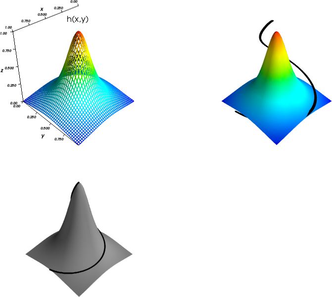
The calls to plt.figure() take three parameters: First the usual index for the plot, then two tuples of numbers ,
representing the RGB-values to be used for the foreground (fgcolor) and the background (bgcolor).
White and black are (1,1,1) and (0,0,0), respectively. The foreground color is used for text and labels included in the plot.
The color attribute in plt.surf adjusts the surface so that it is colored with small variations from the provided base color, here (.5, .5, .5).
The command plot3d is used to plot the curve \( \boldsymbol{r}(t) \). We have here increased the
attribute tube_radius to make the curve thicker and more visible.
Mayavi does no auto-scaling of the axes by default (contrary to Matplotlib),
so if the magnitudes in the vertical and horizontal directions are very different, as they are for \( h(x,y) \),
the plots may be very concentrated in one direction.
We therefore need to apply some auto-scaling procedure.
In Figure 16 two such procedures are exemplified.
In the first two plots the parameter extent is used.
It tells Mayavi to auto-scale the surface and curve to fit the contents described
by the six listed values (we will return to what these values mean when we have a more illustrating example).
Since the curve and the surface span different areas in space, we see that they are auto-scaled differently in the second plot,
with the undesired effect that \( \boldsymbol{r}(t) \) is not drawn on the surface.
The last plot has avoided this problem by using the warp_scale parameter for scaling the vertical direction.
Not all Mayavi functions accept this parameter. A remedy for this is to scale the \( z \)-coordinates manually,
as here exemplified in the last plot3d-call. As is seen, the curve is drawn correctly with respect to the surface in the last plot.
In the following we will use the warp_scale parameter to avoid such auto-scaling problems.
The two plots in Figure 16 were created as separate figures. One can also create them as subplots within one figure:
plt.figure(4, fgcolor=(.0, .0, .0), bgcolor=(1.0, 1.0, 1.0))
plt.mesh(xv, yv, hv, extent=(0, 0.25, 0, 0.25, 0, 0.25),
         colormap='cool')
plt.outline(plt.mesh(
    xv, yv, hv,
    extent=(0.375, 0.625, 0, 0.25, 0, 0.25),
    colormap='Accent'))
plt.outline(plt.mesh(
    xv, yv, hv, extent=(0.75, 1, 0, 0.25, 0, 0.25),
    colormap='prism'), color=(.5, .5, .5))
mesh commands are run, each producing a new plot in the current figure.
The commands use different values for the colormap attribute to color the surface in different ways.
When this attribute is not provided, as in the code producing the two first plots in Figure 16, a default colormap is used.
The plt.outline command is used to create a frame around the
subplots, and as seen, we exemplify this possibility for the last two
subplots, but not the first one. We see that one of the two frames
has a different color, obtained by setting the color attribute of
the plt.outline command.
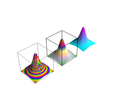
From the computer code it is hopefully clear that the six values listed in extent represent fractions of the cube (0,1,0,1,0,1), where the corresponding plots are placed.
The extents for the three plots are here defined such that they do not overlap.
Figure 17: A plot with three subplots created with Mayavi.
The following code exemplifies how one can produce contour plots with
Mayavi. The code is very similar to that of Matplotlib, but one
difference is that the attribute contours now can represent the
number of levels, as well as the levels themselves.
The plots are shown in Figure 18.
# Default contour plot plotted together with surf.
plt.figure(5, fgcolor=(.0, .0, .0), bgcolor=(1.0, 1.0, 1.0))
plt.surf(xv, yv, hv, warp_scale=0.01)
plt.contour_surf(xv, yv, hv, warp_scale=0.01)

# 10 contour lines (equally spaced contour levels).
plt.figure(6, fgcolor=(.0, .0, .0), bgcolor=(1.0, 1.0, 1.0))
plt.contour_surf(xv, yv, hv, contours=10, warp_scale=0.01)

# 10 contour lines (equally spaced contour levels) together
# with surf. Black color for contour lines.
plt.figure(7, fgcolor=(.0, .0, .0), bgcolor=(1.0, 1.0, 1.0))
plt.surf(xv, yv, hv, warp_scale=0.01)
plt.contour_surf(xv, yv, hv, contours=10, color=(0., 0., 0.),
                 warp_scale=0.01)

# Specify the contour levels explicitly as a list.
plt.figure(8, fgcolor=(.0, .0, .0), bgcolor=(1.0, 1.0, 1.0))
levels = [500., 1000., 1500., 2000.]
plt.contour_surf(xv, yv, hv, contours=levels, warp_scale=0.01)

# View the contours by displaying as an image.
plt.figure(9, fgcolor=(.0, .0, .0), bgcolor=(1.0, 1.0, 1.0))
plt.imshow(hv)
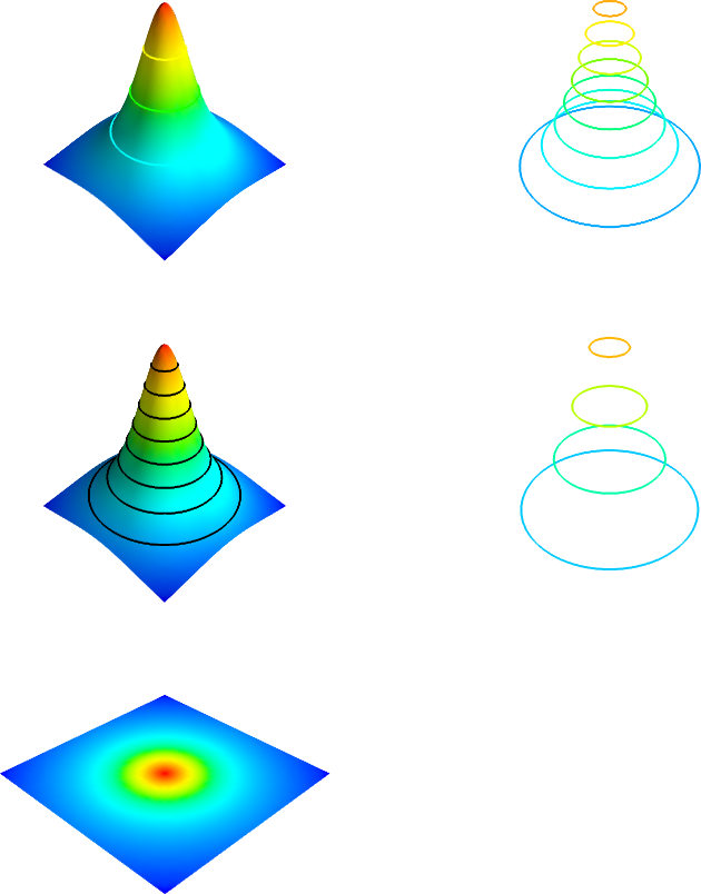
Contour plots in Mayavi are shown in three-dimensional space, but you
can rotate and look at them from above if you want a two-dimensional
plot. Their visual appearance may be enhanced by also including the
surface plot itself. We have done this for the top and middle left plots
in Figure 18.
There is a clear difference in visual impression between these
two plots: in the first one, default surface- and contour coloring is used,
resulting in less visible contours, but in the middle left plot (plt.figure 6), we set black contours to make them better stand out.
Figure 18: Some contour plots with Mayavi.
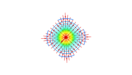
Mayavi supports only vector fields in three-dimensional space. We will therefore visualize the two-dimensional gradient field (15) by adding a third component of zero. The following code plots this gradient field together with the contours of \( h \).
plt.figure(11, fgcolor=(.0, .0, .0), bgcolor=(1.0, 1.0, 1.0))
plt.contour_surf(xv, yv, hv, contours=20, warp_scale=0.01)

# mode controls the style how vectors are drawn
# color controls the colors of the vectors
# scale_mode='none' ensures that vectors are drawn with the same length
plt.quiver3d(x2v, y2v, 0.01*h2v, dhdx, dhdy, np.zeros_like(dhdx),
             mode='arrow', color=(1,0,0), scale_mode='none')
Figure 19: Gradient field with contour plot.
Mayavi has functionality for drawing contour surfaces of 3D scalar fields. Let us consider the 3D scalar field $$ \begin{equation} \tag{16} g(x,y,z) = z-h(x,y). \end{equation} $$ A three-dimensional grid for \( g \) can be computed as follows.
x = y = np.linspace(-10.,10.,41)
z = np.linspace(0, 50, 41)
xv, yv, zv = np.meshgrid(x, y, z,
                         sparse=False, indexing='ij')
hv = 0.01*h0/(1 + (xv**2+yv**2)/(R**2))
gv = zv - hv
A corresponding vector field can be calculated:
$$
\begin{equation}
\nabla g = \frac{\partial g}{\partial x}\boldsymbol{i} + \frac{\partial g}{\partial y}\boldsymbol{j} + \frac{\partial g}{\partial z}\boldsymbol{k}.
\tag{17}
\end{equation}
$$
numpy's gradient function can be used to compute a gradient vector field in
3D as well, but you
need a three-dimensional grid for the field as input.
For the field (16), the gradient field is computed as follows.
x2 = y2 = np.linspace(-10.,10.,5)
z2 = np.linspace(0, 50, 5)
x2v, y2v, z2v = np.meshgrid(x2, y2, z2,
                            indexing='ij', sparse=False)
h2v = 0.01*h0/(1 + (x2v**2 + y2v**2)/(R**2))
g2v = z2v - h2v
dhdx, dhdy, dhdz = np.gradient(g2v)
To visualize the field (16) and its gradient field together, we draw enough contours, as we did in the 2D case in Figure 14. The following code can be used.
plt.figure(12, fgcolor=(.0, .0, .0), bgcolor=(1.0, 1.0, 1.0))
# opacity controls how contours are visible through each other
plt.contour3d(xv, yv, zv, gv, contours=7, opacity=0.5)
# scale_mode='none': vectors should not be scaled
plt.quiver3d(x2v, y2v, z2v, dhdx, dhdy, dhdz, mode='arrow',
             scale_mode='none', opacity=0.5)
Figure 20: The 3D scalar field (16) and its gradient field.
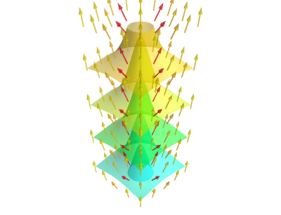
This example demonstrates some of the challenges in plotting three-dimensional vector fields. The vectors must not be too dense, and not too long. It is inevitable that contours shadow one another. Fortunately, Mayavi supports an opacity setting, which controls how contours are visible through each other. Visualizing a 3D scalar field is clearly challenging, and we have only touched the subject.
It is straightforward to create animations with Mayavi. In the following code the function \( h(x,y) \) is scaled vertically, for different scaling constants between \( 0 \) and \( 1 \), and each plot is saved in its own file. The files can then be combined to a standard video file.
plt.figure(13, fgcolor=(.0, .0, .0), bgcolor=(1.0, 1.0, 1.0))
s = plt.surf(xv, yv, hv, warp_scale=0.01)

for i in range(10):
    # s.mlab_source.scalars is a handle for the values of the surface,
    # and is updated here
    s.mlab_source.scalars = hv*0.1*(i+1)
    plt.savefig('tmp_%04d.png' % i)