$$
\newcommand{\tp}{\thinspace .}
$$
This chapter is taken from the book A Primer on Scientific Programming with Python by H. P. Langtangen, 5th edition, Springer, 2016.
Vectors
This section gives a brief introduction to the vector concept,
assuming that you have heard about vectors in the plane and maybe
vectors in space before. This background will be valuable when we
start to work with arrays and curve plotting.
The vector concept
Some mathematical quantities are associated with a set of numbers. One
example is a point in the plane, where we need two coordinates (real
numbers) to describe the point mathematically. Naming the two
coordinates of a particular point as \( x \) and \( y \), it is common to use
the notation \( (x,y) \) for the point. That is, we group the numbers
inside parentheses. Instead of symbols we might use the numbers
directly: \( (0,0) \) and \( (1.5,-2.35) \) are also examples of coordinates
in the plane.
A point in three-dimensional space has three coordinates, which we may
name \( x_1 \), \( x_2 \), and \( x_3 \). The common notation groups the numbers
inside parentheses: \( (x_1,x_2,x_3) \). Alternatively, we may use the
symbols \( x \), \( y \), and \( z \), and write the point as \( (x,y,z) \), or
numbers can be used instead of symbols.
From high school you may have a memory of solving two equations with
two unknowns. At the university you will soon meet problems that are
formulated as \( n \) equations with \( n \) unknowns. The solution of such
problems contains \( n \) numbers that we can collect inside parentheses
and number from 1 to \( n \): \( (x_1,x_2,x_3,\ldots,x_{n-1},x_n) \).
Quantities such as \( (x,y) \), \( (x,y,z) \), or \( (x_1,\ldots,x_n) \) are known
as vectors in mathematics. A visual representation of a vector is
an arrow that goes from the origin to a point. For example, the vector
\( (x,y) \) is an arrow that goes from \( (0,0) \) to the point with
coordinates \( (x,y) \) in the plane. Similarly, \( (x,y,z) \) is an arrow
from \( (0,0,0) \) to the point \( (x,y,z) \) in three-dimensional space.
Mathematicians found it convenient to introduce spaces with higher
dimension than three, because when we have a solution of \( n \) equations
collected in a vector \( (x_1,\ldots,x_n) \), we may think of this vector
as a point in a space with dimension \( n \), or equivalently, an arrow
that goes from the origin \( (0,\ldots,0) \) in \( n \)-dimensional space to
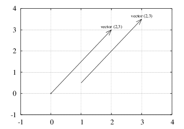
the point \( (x_1,\ldots,x_n) \). Figure 1
illustrates a vector as an arrow, either starting at the origin, or at
any other point. Two arrows/vectors that have the same direction and
the same length are mathematically equivalent.
Figure 1: A vector \( (2,3) \) visualized in the standard way as an arrow from the origin to the point \( (2,3) \), and mathematically equivalently, as an arrow from \( (1,\frac{1}{2}) \) (or any point \( (a,b) \)) to \( (3, 3\frac{1}{2}) \) (or \( (a+2,b+3) \)).
We say that \( (x_1,\ldots,x_n) \) is an \( n \)-vector or a vector with \( n \)
components. Each of the numbers \( x_1 \), \( x_2 \), \( \ldots \) is a component
or an element. We refer to the first component (or element), the
second component (or element), and so forth.
A Python program may use a list or tuple to represent a vector:
v1 = [x, y]         # list of variables
v2 = (-1, 2)        # tuple of numbers
v3 = (x1, x2, x3)   # tuple of variables
from math import exp
v4 = [exp(-i*0.1) for i in range(150)]
While v1 and v2 are vectors in the plane and v3 is a vector in
three-dimensional space, v4 is a vector in a 150-dimensional space,
consisting of 150 values of the exponential function. Since Python
lists and tuples have 0 as the first index, we may also in mathematics
write the vector \( (x_1,x_2) \) as \( (x_0,x_1) \). This is not at all common
in mathematics, but makes the distance from a mathematical description
of a problem to its solution in Python shorter.
It is impossible to visually demonstrate how a space with 150
dimensions looks like. Going from the plane to three-dimensional
space gives a rough feeling of what it means to add a dimension, but
if we forget about the idea of a visual perception of space, the
mathematics is very simple: going from a 4-dimensional vector to a
5-dimensional vector is just as easy as adding an element to a list of
symbols or numbers.
Mathematical operations on vectors
Since vectors can be viewed as arrows having a length and a direction,
vectors are extremely useful in geometry and physics. The velocity of
a car has a magnitude and a direction, so has the acceleration, and
the position of a point in the car is also a vector. An edge of a
triangle can be viewed as a line (arrow) with a direction and length.
In geometric and physical applications of vectors, mathematical
operations on vectors are important. We shall exemplify some of the
most important operations on vectors below. The goal is not to teach
computations with vectors, but more to illustrate that such
computations are defined by mathematical rules. Given two vectors,
\( (u_1,u_2) \) and \( (v_1,v_2) \), we can add these vectors according to the
rule:
$$
\begin{equation}
(u_1,u_2) + (v_1,v_2) = (u_1+v_1, u_2+v_2)\tp
\tag{1}
\end{equation}
$$
We can also subtract two vectors using a similar rule:
$$
\begin{equation}
(u_1,u_2) - (v_1,v_2) = (u_1-v_1, u_2-v_2)\tp
\tag{2}
\end{equation}
$$
A vector can be multiplied by a number. This number, called \( a \) below, is
usually denoted as a scalar:
$$
\begin{equation}
a\cdot (v_1,v_2) = (av_1, av_2)\tp
\tag{3}
\end{equation}
$$
The inner product, also called dot product, or scalar product,
of two vectors is a number:
$$
\begin{equation} (u_1,u_2)\cdot (v_1,v_2) = u_1v_1 + u_2v_2\tp
\tag{4}
\end{equation}
$$
(From high school mathematics and physics you might recall that the
inner or dot product also can be expressed as the product of the
lengths of the two vectors multiplied by the cosine of the angle
between them, but we will not make use of that formula. There is also
a cross product defined for 2-vectors or 3-vectors, but we do not
list the cross product formula here.)
The length of a vector is defined by
$$
\begin{equation} ||(v_1,v_2)|| = \sqrt{(v_1,v_2)\cdot (v_1,v_2)}= \sqrt{v_1^2 + v_2^2}\tp
\tag{5}
\end{equation}
$$
The same mathematical operations apply to \( n \)-dimensional vectors as
well. Instead of counting indices from 1, as we usually do in
mathematics, we now count from 0, as in Python. The addition and
subtraction of two vectors with \( n \) components (or elements) read
$$
\begin{align}
(u_0,\ldots,u_{n-1}) + (v_0,\ldots,v_{n-1}) &= (u_0+v_0,\ldots,u_{n-1}+v_{n-1}) ,
\tag{6}\\
(u_0,\ldots,u_{n-1}) - (v_0,\ldots,v_{n-1}) &= (u_0-v_0,\ldots,u_{n-1}-v_{n-1}) \tp
\tag{7}
\end{align}
$$
Multiplication of a scalar \( a \) and a vector \( (v_0,\ldots,v_{n-1}) \) equals
$$
\begin{equation}
(av_0,\ldots,av_{n-1})\tp
\tag{8}
\end{equation}
$$
The inner or dot product of two \( n \)-vectors is defined as
$$
\begin{equation}
(u_0,\ldots,u_{n-1}) \cdot (v_0,\ldots,v_{n-1})
= u_0v_0+\cdots + u_{n-1}v_{n-1} = \sum_{j=0}^{n-1} u_jv_j\tp
\tag{9}
\end{equation}
$$
Finally, the length \( ||v|| \) of an \( n \)-vector \( v=(v_0,\ldots,v_{n-1}) \) is
$$
\begin{align}
\sqrt{(v_0,\ldots,v_{n-1})\cdot (v_0,\ldots,v_{n-1})} &=
\left(v_0^2 + v_1^2 + \cdots + v_{n-1}^2\right)^\frac{1}{2}\nonumber\\
& =
\left(\sum_{j=0}^{n-1} v_j^2\right)^\frac{1}{2}\tp
\tag{10}
\end{align}
$$
Vector arithmetics and vector functions
In addition to the operations on vectors in the section Mathematical operations on vectors, which you might recall from high school
mathematics, we can define other operations on vectors. This is very
useful for speeding up programs. Unfortunately, the forthcoming
vector operations are hardly treated in textbooks on mathematics, yet
these operations play a significant role in mathematical software,
especially in computing environment such as MATLAB, Octave, Python,
and R.
Applying a mathematical function of one variable, \( f(x) \), to a vector
is defined as a vector where \( f \) is applied to each element. Let
\( v=(v_0,\ldots,v_{n-1}) \) be a vector. Then
$$
\begin{equation*} f(v) = (f(v_0),\ldots,f(v_{n-1}))\tp\end{equation*}
$$
For example, the sine of \( v \) is
$$
\begin{equation*} \sin(v) = (\sin(v_0),\ldots,\sin(v_{n-1}))\tp\end{equation*}
$$
It follows that squaring a vector, or the more general operation of
raising the vector to a power, can be defined as applying the
operation to each element:
$$
\begin{equation*} v^b = (v_0^b,\ldots,v_{n-1}^b)\tp\end{equation*}
$$
Another operation between two vectors that arises in computer programming
of mathematics is the "asterisk" multiplication, defined as
$$
\begin{equation} u*v = (u_0v_0, u_1v_1, \ldots, u_{n-1}v_{n-1})\tp
\tag{11}
\end{equation}
$$
Adding a scalar to a vector or array can be defined as adding the scalar
to each component. If \( a \) is a scalar and \( v \) a vector, we have
$$
\begin{equation*} a + v = (a+v_0, \ldots, a+v_{n-1})\tp\end{equation*}
$$
A compound vector expression may look like
$$
\begin{equation}
v^2*\cos(v)*e^v + 2\tp
\tag{12}
\end{equation}
$$
How do we calculate this expression? We use the normal rules of
mathematics, working our way, term by term, from left to right, paying
attention to the fact that powers are evaluated before multiplications
and divisions, which are evaluated prior to addition and subtraction.
First we calculate \( v^2 \), which results in a vector we may call
\( u \). Then we calculate \( \cos(v) \) and call the result \( p \). Then we
multiply \( u*p \) to get a vector which we may call \( w \). The next step is
to evaluate \( e^v \), call the result \( q \), followed by the multiplication
\( w*q \), whose result is stored as \( r \). Then we add \( r+2 \) to get the
final result. It might be more convenient to list these operations
after each other:
- \( u=v^2 \)
- \( p=\cos (v) \)
- \( w = u*p \)
- \( q = e^v \)
- \( r = w*q \)
- \( s=r +2 \)
Writing out the vectors \( u \), \( w \), \( p \), \( q \), and \( r \) in terms of a
general vector \( v=(v_0,\ldots,v_{n-1}) \) (do it!) shows that the result
of the expression (12) is the vector
$$
\begin{equation*} (v_0^2\cos(v_0)e^{v_0}+2,\ldots,v_{n-1}^2\cos(v_{n-1})e^{v_{n-1}}+2)\tp\end{equation*}
$$
That is, component no. \( i \) in the result vector equals the number
arising from applying the formula (12) to \( v_i \),
where the * multiplication is ordinary multiplication between two
numbers.
We can, alternatively, introduce the function
$$
\begin{equation*} f(x) = x^2\cos(x)e^x + 2\end{equation*}
$$
and use the result that \( f(v) \)
means applying \( f \) to each element
in \( v \). The result is the same as in the vector
expression (12).
In Python programming it is important for speed (and convenience too)
that we can apply functions of one variable, like \( f(x) \), to
vectors. What this means mathematically is something we have tried to
explain in this subsection. Doing Exercise 5: Apply a function to a vector
and Exercise 6: Simulate by hand a vectorized expression may help to grasp the ideas of vector computing,
and with more programming experience you will hopefully discover that
vector computing is very useful. It is not necessary to have a
thorough understanding of vector computing in order to proceed with
the next sections.
Arrays are used to represent vectors in a program, but one can do more
with arrays than with vectors. Until the section Higher-dimensional arrays it
suffices to think of arrays as the same as vectors in a program.