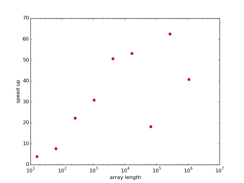
Figure 11: Improved efficiency of vectorizing the "axpy" operation as function of array length.
This chapter is taken from the book A Primer on Scientific Programming with Python by H. P. Langtangen, 5th edition, Springer, 2016.
This section lists some more advanced but useful operations with Numerical Python arrays.
Let x be an array. The statement a = x makes a refer to the same
array as x. Changing a will then also affect x:
>>> import numpy as np
>>> x = np.array([1, 2, 3.5])
>>> a = x
>>> a[-1] = 3  # this changes x[-1] too!
>>> x
array([ 1.,  2.,  3.])
a without changing x requires a to be a copy of x:
>>> a = x.copy()
>>> a[-1] = 9
>>> a
array([ 1.,  2.,  9.])
>>> x
array([ 1.,  2.,  3.])
Let a and b be two arrays of the same shape. The expression a +=
b means a = a + b, but this is not the complete story. In the
statement a = a + b, the sum a + b is first computed, yielding a
new array, and then the name a is bound to this new array. The old
array a is lost unless there are other names assigned to this array.
In the statement a += b, elements of b are added directly into the
elements of a (in memory). There is no hidden intermediate array as
in a = a + b. This implies that a += b is more efficient than a
= a + b since Python avoids making an extra array. We say that the
operators +=, *=, and so on, perform in-place arithmetics in
arrays.
Consider the compound array expression
a = (3*x**4 + 2*x + 4)/(x + 1)
r1 = x**4r2 = 3*r1r3 = 2*xr4 = r2 + r3r5 = r4 + 4r6 = x + 1r7 = r5/r6a = r7
a = x.copy()
a **= 4
a *= 3
a += 2*x
a += 4
a /= x + 1
x, and computing the right-hand sides 2*x and x+1.
Quite often in computational science and engineering, a huge number of arithmetics is performed on very large arrays, and then saving memory and array allocation time by doing in-place arithmetics is important.
The mix of assignment and in-place arithmetics makes it easy to make
unintended changes of more than one array. For example, this code
changes x:
a = x
a += y
a refers to the same array as x and the change of
a is done in-place.
We have already seen that the np.zeros function is handy for making
a new array a of a given size. Very often the size and the type of
array elements have to match another existing array x. We can then
either copy the original array, e.g.,
a = x.copy()
a with the right new values, or we can
say
a = np.zeros(x.shape, x.dtype)
x.dtype holds the array element type (dtype for
data type), and x.shape is a tuple with
the array dimensions. The variable a.ndim holds the number of
dimensions.
Sometimes we may want to ensure that an object is an array, and if
not, turn it into an array. The np.asarray function is useful in
such cases:
a = np.asarray(a)
a already is an array, but if a is a list
or tuple, a new array with a copy of the data is created.
The section Basics of numerical Python arrays shows how slices can be used to
extract and manipulate subarrays. The slice f:t:i corresponds to
the index set f, f+i, f+2*i, ... up to, but not including, t.
Such an index set can be given explicitly too: a[range(f,t,i)].
That is, the integer list from range can be used as a set of
indices. In fact, any integer list or integer array can be used as
index:
>>> a = np.linspace(1, 8, 8)
>>> a
array([ 1.,  2.,  3.,  4.,  5.,  6.,  7.,  8.])
>>> a[[1,6,7]] = 10
>>> a
array([  1.,  10.,   3.,   4.,   5.,   6.,  10.,  10.])
>>> a[range(2,8,3)] = -2   # same as a[2:8:3] = -2
>>> a
array([  1.,  10.,  -2.,   4.,   5.,  -2.,  10.,  10.])
True values. This functionality allows expressions like
a[x<m]. Here are two examples, continuing the previous interactive
session:
>>> a[a < 0]            # pick out the negative elements of a
array([-2., -2.])
>>> a[a < 0] = a.max()
>>> a
array([  1.,  10.,  10.,   4.,   5.,  10.,  10.,  10.])
>>> # Replace elements where a is 10 by the first
>>> # elements from another array/list:
>>> a[a == 10] = [10, 20, 30, 40, 50, 60, 70]
>>> a
array([  1.,  10.,  20.,   4.,   5.,  30.,  40.,  50.])
Inside an interactive Python shell you can easily check an object's type
using the type
In case of a Numerical Python array, the type name is ndarray:
>>> a = np.linspace(-1, 1, 3)
>>> a
array([-1.,  0.,  1.])
>>> type(a)
<type 'numpy.ndarray'>
ndarray or a float
or int. The isinstance function can be used this purpose:
>>> isinstance(a, np.ndarray)
True
>>> isinstance(a, (float,int))  # float or int?
False
isinstance and type to check on object's type is
shown next.
Suppose we have a constant function,
def f(x):
    return 2
x, but will return a float
while a vectorized version of the function should return an array of
the same shape as x where each element has the value 2. The
vectorized version can be realized as
def fv(x):
    return np.zeros(x.shape, x.dtype) + 2
def f(x):
    if isinstance(x, (float, int)):
        return 2
    elif isinstance(x, np.ndarray):
        return np.zeros(x.shape, x.dtype) + 2
    else:
        raise TypeError\
        ('x must be int, float or ndarray, not %s' % type(x))
There is a special compact syntax r_[f:t:s] for the linspace
function:
>>> a = r_[-5:5:11j]  # same as linspace(-5, 5, 11)
>>> print a
[-5. -4. -3. -2. -1.  0.  1.  2.  3.  4.  5.]
11j means 11 coordinates (between -5 and 5, including the
upper limit 5). That is, the number of elements in the array is given
with the imaginary number syntax.
The shape attribute in array objects holds the shape, i.e., the size
of each dimension. A function size returns the total number of
elements in an array. Here are a few equivalent ways of changing the
shape of an array:
>>> a = np.linspace(-1, 1, 6)
>>> print a
[-1.  -0.6 -0.2  0.2  0.6  1. ]
>>> a.shape
(6,)
>>> a.size
6
>>> a.shape = (2, 3)
>>> a = a.reshape(2, 3)    # alternative
>>> a.shape
(2, 3)
>>> print a
[[-1.  -0.6 -0.2]
 [ 0.2  0.6  1. ]]
>>> a.size                 # total no of elements
6
>>> len(a)                 # no of rows
2
>>> a.shape = (a.size,)    # reset shape
len(a) always returns the length of the first
dimension of an array.
Programs with lots of array calculations may soon consume much time and memory, so it may quickly become crucial to speed up calculations and use as little memory as possible. The main technique for speeding up array calculations is vectorization, i.e., avoiding explicit loops in Python over array elements. To save memory usage, one needs to understand when arrays get allocated and avoid this by in-place array arithmetics.
axpy Our computational case study concerns the famous "axpy" operation: \( r = ax + y \), where \( a \) is a number and \( x \) and \( y \) are arrays. All implementations and the associated experimentation are found in the file hpc_axpy.py.
A naive loop implementation of the "axpy" operation \( ax+y \) reads
def axpy_loop_newr(a, x, y):
    r = np.zeros_like(x)
    for i in range(r.size):
        r[i] = a*x[i] + y[i]
    return r
Classical implementations overwrite \( y \) by \( ax + y \): \( y \leftarrow ax+y \), but we shall make implementations where we either can overwrite \( y \) or place \( ax+y \) in another array. The function above creates a new array for the result.
Rather than allocating the array inside the function, we can put that
burden on the user and provide a result array r as input:
def axpy_loop(a, x, y, r):
    for i in range(r.size):
        r[i] = a*x[i] + y[i]
    return r
# Classical axpy
y = axpy_loop(a, x, y, y)

# Store axpy result in separate array
r = np.zeros_like(x)
r = axpy_loop(a, x, y, r)
The call
r = axpy_loop(a, x, y, r)
axpy_loop(a, x, y, r)
r is then
transferred as a reference or pointer to the array data).
In Python, there is no need for the function axpy_loop to return r, because
the assignment to r[i] inside the loop changes all elements of the
r. The array r will therefore be modified after calling
axpy_loop(a, x, y, r) anyway. However, it is a good convention in Python
that all input data to a function are arguments and all output data
are returned. With
r = axpy_loop(a, x, y, r)
r is both input and output.
The vectorized implementation of the "axpy" operation reads
def axpy1(a, x, y):
    r = a*x + y
    return r
r arising from the
operation a*x+y.
The speed up of vectorization is significant, see
Figure 11 (made by the function effect_of_vec
in the file hpc_axpy.py).
Figure 11: Improved efficiency of vectorizing the "axpy" operation as function of array length.
Temporary arrays are needed in the vectorized implementation.
One would expect that a*x must be calculated and stored in
a temporary array, call it r1, and then r1 + y must be
evaluated and stored in another allocated array r, which is returned.
It appears that a*x + y only needs the allocation of one array,
the one to be returned (we have investigated the memory consumption
in detail using the memory_profiler module). Anyway, repeated
calls to axpy1 with large arrays lead to an allocation of a new
large array in each call.
Applications with large arrays should avoid unnecessary allocation
of temporary arrays and instead reuse pre-allocated arrays.
Suppose we have allocated an array for the result r = ax + y once
and for all. We can pass the r array to the computing function
as in the axpy_loop function above and use the memory in r
for intermediate calculation. In vectorized code, this requires
use of in-place array
arithmetics. For example, u += v adds each element in v into
u. The mathematically equivalent construction u = u + v would
first create an object from u + v and then assign the name u
to this object. Similarly, u *= a multiplies all elements in u
by the number a. Other in-place operators are -= for
elementwise subtraction,
/= for elementwise division, and **= for elementwise exponentiation.
In-place arithmetics for doing r = a*x + y in a pre-allocated
array r will first copy all elements of x into r, then
perform elementwise multiplication by a, and finally elementwise
addition of y:
def axpy2(a, x, y, r):
    r[:] = x
    r *= a
    r += y
    return r
r[:] = x inserts the elements of x into r.
A mathematically equivalent construction, r = x.copy(), allocates
a new object and fills it with the values of x before the name
r refers to this object. The array r supplied as argument to the
function is then lost, and the returned array is another object.
We can perform repeated calls to the axpy2 function without any
extra memory allocation. This can be proved by a small code snippet
where we use id(r) to see the unique identity of the r array.
If this identity remains constant through calls, we always reuse
the pre-allocated r array:
r = np.zeros_like(x)
print id(r)
for i in range(10):
    r = axpy2(a, x, y, r)
    print id(r)
r to axpy2 that is also returned.
We can equally well drop returning r and utilize that the changes
made by in-place arithmetics is always reflected in the r array
we allocate outside the function:
def axpy3(a, x, y, r):
    r[:] = x
    r *= a
    r += y
axpy3(a, x, y, r)
The module memory_profiler is very useful for analyzing the memory
usage of every statement in a program. The module is installed
by
Terminal> sudo pip install memory_profiler
@profile at the line above, e.g.,
@profile
def axpy1(a, x, y:
    r = a*x + y
    return r
axpy.py by
Terminal> python -m memory_profiler axpy.py
Line #    Mem usage    Increment   Line Contents
================================================
     1  251.977 MiB    0.000 MiB   @profile
     2                             def axpy1(a, x, y:
     3  328.273 MiB   76.297 MiB       r = a*x + y
     4  328.273 MiB    0.000 MiB       return r

Line #    Mem usage    Increment   Line Contents
================================================
     6  251.977 MiB    0.000 MiB   @profile
     7                             def axpy2(a, x, y, r):
     8  251.977 MiB    0.000 MiB       r[:] = x
     9  251.977 MiB    0.000 MiB       r *= a
    10  251.977 MiB    0.000 MiB       r += y
    11  251.977 MiB    0.000 MiB       return r
axpy1 compared
with axpy2.
The module line_profiler can time each line of a program.
Installation is easily done by sudo pip install line_profiler.
As for module_profiler described in the previous section,
also line_profiler requires each function to be analyzed to
have (the decorator) @profile at the line above the function.
The module is installed together with an analysis script
kernprof that we use to run the program:
Terminal> kernprof -l -v axpy.py
Total time: 0.014291 s
Function: axpy1 at line 1

Line #  Hits     Time  Per Hit   % Time  Line Contents
==============================================================
 1                                       @profile
 2                                       def axpy1(a, x, y):
 3     3        14283   4761.0     99.9      r = a*x + y
 4     3            8      2.7      0.1      return r

Total time: 0.004382 s
Function: axpy2 at line 6

Line #  Hits  Time  Per Hit   % Time  Line Contents
==============================================================
 6                                    @profile
 7                                    def axpy2(a, x, y, r):
 8     3      1981    660.3     45.2      r[:] = x
 9     3      1258    419.3     28.7      r *= a
10     3      1138    379.3     26.0      r += y
11     3         5      1.7      0.1      return r

Total time: 1.38674 s
Function: axpy_loop at line 26

Line #  Hits    Time Per Hit  % Time  Line Contents
==============================================================
26                                    @profile
27                                    def axpy_loop(a, x, y, r):
28   1500006  449747     0.3    32.4      for i in range(r.size):
29   1500003  936985     0.6    67.6          r[i] = a*x[i] + y[i]
30         3      10     3.3     0.0      return r
Both line_profiler and memory_profiler are very useful tools
for spotting inefficient constructions in a code.