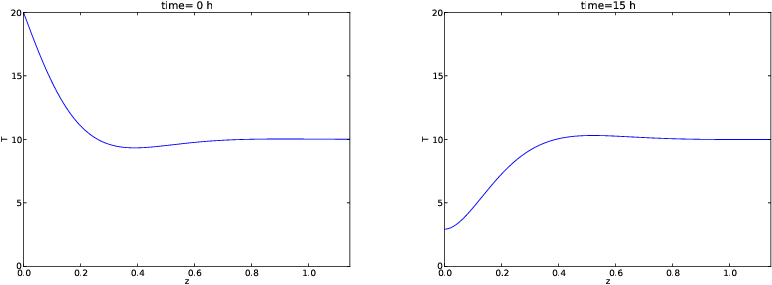
Figure 21: Plot of the temperature \( T(z,t) \) in the ground for two different \( t \) values.
This chapter is taken from the book A Primer on Scientific Programming with Python by H. P. Langtangen, 5th edition, Springer, 2016.
This document has introduced computing with arrays and plotting curve data stored in arrays. The Numerical Python package contains lots of functions for array computing, including the ones listed in the table below. Plotting has been done with tools that closely resemble the syntax of MATLAB.
| Construction | Meaning |
|---|---|
array(ld) | copy list data ld to a numpy array |
asarray(d) | make array of data d (no data copy if already array) |
zeros(n) | make a float vector/array of length n, with zeros |
zeros(n, int) | make an int vector/array of length n with zeros |
zeros((m,n)) | make a two-dimensional float array with shape (m,`n`) |
zeros_like(x) | make array of same shape and element type as x |
linspace(a,b,m) | uniform sequence of m numbers in \( [a,b] \) |
a.shape | tuple containing a's shape |
a.size | total no of elements in a |
len(a) | length of a one-dim. array a (same as a.shape[0]) |
a.dtype | the type of elements in a |
a.reshape(3,2) | return a reshaped as \( 3\times 2 \) array |
a[i] | vector indexing |
a[i,j] | two-dim. array indexing |
a[1:k] | slice: reference data with indices 1,2,...,k-1 |
a[1:10:3] | slice: reference data with indices 1,4,7 |
b = a.copy() | copy an array |
sin(a), exp(a), ... | numpy functions applicable to arrays |
c = concatenate((a, b)) | c contains a with b appended |
c = where(cond, a1, a2) | c[i] = a1[i] if cond[i], else c[i] = a2[i] |
isinstance(a, ndarray) | is True if a is an array |
When we apply a Python function f(x) to a Numerical Python array
x, the result is the same as if we apply f to each element in x
separately. However, when f contains if statements, these are in
general invalid if an array x enters the boolean expression. We
then have to rewrite the function, often by applying the where
function from Numerical Python.
The sections MATLAB-style plotting with Matplotlib and Matplotlib; pyplot prefix provide a quick overview of how to plot curves with the aid of Matplotlib. The same examples coded with the Easyviz plotting interface appear in the section SciTools and Easyviz.
Each frame in a movie must be a hardcopy of a plot in PNG format.
These plot files should have names containing a counter padded with
leading zeros. One example may be tmp_0000.png, tmp_0001.png,
tmp_0002.png. Having the plot files with names on this form, we can
make an animated GIF movie in the file movie.gif, with two frames
per second, by
os.system('convert -delay 50 tmp_*.png movie.gif')
os.system('ffmpeg -r 5 -i tmp_%04d.png -vcodec flv movie.flv')
The important topics in this document are
In this document's summarizing example we shall visualize how the temperature varies downward in the earth as the surface temperature oscillates between high day and low night values. One question may be: What is the temperature change 10 m down in the ground if the surface temperature varies between 2 C in the night and 15 C in the day?
Let the \( z \) axis point downwards, towards the center of the earth, and let \( z=0 \) correspond to the earth's surface. The temperature at some depth \( z \) in the ground at time \( t \) is denoted by \( T(z,t) \). If the surface temperature has a periodic variation around some mean value \( T_0 \), according to $$ \begin{equation*} T(0,t)=T_0+ A\cos (\omega t),\end{equation*} $$ one can find, from a mathematical model for heat conduction, that the temperature at an arbitrary depth is $$ \begin{equation} T(z,t) = T_0 + Ae^{-az}\cos (\omega t - az),\quad a =\sqrt{\omega\over 2k}\tp \tag{18} \end{equation} $$ The parameter \( k \) reflects the ground's ability to conduct heat (\( k \) is called the thermal diffusivity or the heat conduction coefficient).
The task is to make an animation of how the temperature profile in the ground, i.e., \( T \) as a function of \( z \), varies in time. Let \( \omega \) correspond to a time period of 24 hours. The mean temperature \( T_0 \) is taken as 10 C, and the maximum variation \( A \) is assumed to be 10 C. The heat conduction coefficient \( k \) may be set as \( 1\hbox{ mm}^2/\hbox{s} \) (which is \( 10^{-6} \hbox{ m}^2/\hbox{s} \) in proper SI units).
To animate \( T(z,t) \) in time, we need to make a loop over points in time, and in each pass in the loop we must save a plot of \( T \), as a function of \( z \), to file. The plot files can then be combined to a movie. The algorithm becomes
animate function where we just feed
in some \( f(x,t) \) function and make all the plot files. If animate
has arguments for setting the labels on the axis and the extent of the
\( y \) axis, we can easily use animate also for a function \( T(z,t) \) (we
just use \( z \) as the name for the \( x \) axis and \( T \) as the name for the
\( y \) axis in the plot). Recall that it is important to fix the extent
of the \( y \) axis in a plot when we make animations, otherwise most
plotting programs will automatically fit the extent of the axis to the
current data, and the tick marks on the \( y \) axis will jump up and down
during the movie. The result is a wrong visual impression of the
function.
The names of the plot files must have a common stem appended with some
frame number, and the frame number should have a fixed number of
digits, such as 0001, 0002, etc. (if not, the sequence of the plot
files will not be correct when we specify the collection of files with
an asterisk for the frame numbers, e.g., as in tmp*.png). We
therefore include an argument to animate for setting the name stem
of the plot files. By default, the stem is tmp_, resulting in the
filenames tmp_0000.png, tmp_0001.png, tmp_0002.png, and so
forth. Other convenient arguments for the animate function are the
initial time in the plot, the time lag \( \Delta t \) between the plot
frames, and the coordinates along the \( x \) axis. The animate
function then takes the form
def animate(tmax, dt, x, function, ymin, ymax, t0=0,
            xlabel='x', ylabel='y', filename='tmp_'):
    t = t0
    counter = 0
    while t <= tmax:
        y = function(x, t)
        plot(x, y, '-',
             axis=[x[0], x[-1], ymin, ymax],
             title='time=%2d h' % (t/3600.0),
             xlabel=xlabel, ylabel=ylabel,
             savefig=filename + '%04d.png' % counter)
        savefig('tmp_%04d.pdf' % counter)
        t += dt
        counter += 1
The \( T(z,t) \) function is easy to implement, but we need to decide
whether the parameters \( A \), \( \omega \), \( T_0 \), and \( k \) shall be
arguments to the Python implementation of \( T(z,t) \) or if they shall be
global variables. Since the animate function expects that the
function to be plotted has only two arguments, we must implement
\( T(z,t) \) as T(z,t) in Python and let the other parameters be global
variables
(or one can let T be a class with the parameters as attributes
and a method __call__(self, x, t)).
The T(z,t) implementation
then reads
def T(z, t):
    # T0, A, k, and omega are global variables
    a = sqrt(omega/(2*k))
    return T0 + A*exp(-a*z)*cos(omega*t - a*z)
Suppose we plot \( T(z,t) \) at \( n \) points for \( z\in [0,D] \). We make such plots for \( t\in [0,t_{\max}] \) with a time lag \( \Delta t \) between the them. The frames in the movie are now made by
# set T0, A, k, omega, D, n, tmax, dt
z = linspace(0, D, n)
animate(tmax, dt, z, T, T0-A, T0+A, 0, 'z', 'T')
The call to animate above creates a set of files with names
of the form tmp_*.png. Out of these files we can create an
animated GIF movie or a video in, e.g., Flash format by
running operating systems commands with convert and avconv (or
ffmpeg):
os.system('convert -delay 50 tmp_*.png movie.gif')
os.system('avconv -i tmp_%04d.png -r 5 -vcodec flv movie.flv')
It now remains to assign proper values to all the global variables in
the program: n, D, T0, A, omega, dt, tmax, and k. The
oscillation period is 24 hours, and \( \omega \) is related to the period
\( P \) of the cosine function by \( \omega = 2\pi /P \) (realize that \( \cos
(t2\pi/P) \) has period \( P \)). We then express \( P=24 \) h as \( 24\cdot
60\cdot 60 \) s and compute \( \omega \) as \( 2\pi/P \approx 7\cdot
10^{-5}\hbox{ s}^{-1} \). The total simulation time can be 3 periods,
i.e., \( t_{\max} = 3P \). The \( T(z,t) \) function decreases exponentially
with the depth \( z \) so there is no point in having the maximum depth
\( D \) larger than the depth where \( T \) is visually zero, say 0.001. We
have that \( e^{-aD}=0.001 \) when \( D=-a^{-1}\ln 0.001 \), so we can use
this estimate in the program. The proper initialization of all
parameters can then be expressed as follows:
k = 1E-6        # thermal diffusivity (in m*m/s)
P = 24*60*60.   # oscillation period of 24 h (in seconds)
omega = 2*pi/P
dt = P/24       # time lag: 1 h
tmax = 3*P      # 3 day/night simulation
T0 = 10         # mean surface temperature in Celsius
A = 10          # amplitude of the temperature variations in Celsius
a = sqrt(omega/(2*k))
D = -(1/a)*log(0.001) # max depth
n = 501         # no of points in the z direction
We encourage you to run the program
heatwave.py to see the
movie. The hardcopy of the movie is in the file movie.gif.
Figure 21 displays two snapshots in time of
the \( T(z,t) \) function.
Figure 21: Plot of the temperature \( T(z,t) \) in the ground for two different \( t \) values.
In this example, as in many other scientific problems, it was easier to write the code than to assign proper physical values to the input parameters in the program. To learn about the physical process, here how heat propagates from the surface and down in the ground, it is often advantageous to scale the variables in the problem so that we work with dimensionless variables. Through the scaling procedure we normally end up with much fewer physical parameters that must be assigned values. Let us show how we can take advantage of scaling the present problem.
Consider a variable \( x \) in a problem with some dimension. The idea of scaling is to introduce a new variable \( \bar x = x/x_c \), where \( x_c \) is a characteristic size of \( x \). Since \( x \) and \( x_c \) have the same dimension, the dimension cancels in \( \bar x \) such that \( \bar x \) is dimensionless. Choosing \( x_c \) to be the expected maximum value of \( x \), ensures that \( \bar x\leq 1 \), which is usually considered a good idea. That is, we try to have all dimensionless variables varying between zero and one. For example, we can introduce a dimensionless \( z \) coordinate: \( \bar z= z/D \), and now \( \bar z \in [0,1] \). Doing a proper scaling of a problem is challenging so for now it is sufficient to just follow the steps below - and not worry why we choose a certain scaling.
In the present problem we introduce these dimensionless variables: $$ \begin{align*} \bar z &= z/D\\ \bar T &= {T-T_0\over A}\\ \bar t &= {\omega t} \end{align*} $$ We now insert \( z=\bar z D \) and \( t=\bar t/\omega \) in the expression for \( T(z,t) \) and get $$ \begin{equation*} T = T_0 + Ae^{-b\bar z}\cos(\bar t - b\bar z),\quad b=aD\end{equation*} $$ or $$ \begin{equation*} \bar T(\bar z,\bar t) = {T-T_0\over A} = e^{-b\bar z}\cos(\bar t - b\bar z)\tp\end{equation*} $$ We see that \( \bar T \) depends on only one dimensionless parameter \( b \) in addition to the independent dimensionless variables \( \bar z \) and \( \bar t \). It is common practice at this stage of the scaling to just drop the bars and write $$ \begin{equation} T(z,t) = e^{-bz}\cos(t - bz)\tp \tag{19} \end{equation} $$ This function is much simpler to plot than the one with lots of physical parameters, because now we know that \( T \) varies between \( -1 \) and 1, \( t \) varies between 0 and \( 2\pi \) for one period, and \( z \) varies between 0 and 1. The scaled temperature has only one parameter \( b \) in addition to the independent variable. That is, the shape of the graph is completely determined by \( b \).
In our previous movie example, we used specific values for \( D \), \( \omega \), and \( k \), which then implies a certain \( b=D\sqrt{\omega /(2k)} \) (\( \approx 6.9 \)). However, we can now run different \( b \) values and see the effect on the heat propagation. Different \( b \) values will in our problems imply different periods of the surface temperature variation and/or different heat conduction values in the ground's composition of rocks. Note that doubling \( \omega \) and \( k \) leaves the same \( b \) - it is only the fraction \( \omega/k \) that influences the value of \( b \).
We can reuse the animate function also in the scaled case, but
we need to make a new \( T(z,t) \) function and, e.g., a main program
where \( b \) can be read from the command line:
def T(z, t):
    return exp(-b*z)*cos(t - b*z)  # b is global

b = float(sys.argv[1])
n = 401
z = linspace(0, 1, n)
animate(3*2*pi, 0.05*2*pi, z, T, -1.2, 1.2, 0, 'z', 'T')
movie('tmp_*.png', encoder='convert', fps=2,
      output_file='tmp_heatwave.gif')
os.system('convert -delay 50 tmp_*.png movie.gif')
Running the program, found as the file heatwave_scaled.py, for different \( b \) values shows that \( b \) governs how deep the temperature variations on the surface \( z=0 \) penetrate. A large \( b \) makes the temperature changes confined to a thin layer close to the surface, while a small \( b \) leads to temperature variations also deep down in the ground. You are encouraged to run the program with \( b=2 \) and \( b=20 \) to experience the major difference, or just view the ready-made animations.
We can understand the results from a physical perspective. Think of increasing \( \omega \), which means reducing the oscillation period so we get a more rapid temperature variation. To preserve the value of \( b \) we must increase \( k \) by the same factor. Since a large \( k \) means that heat quickly spreads down in the ground, and a small \( k \) implies the opposite, we see that more rapid variations at the surface requires a larger \( k \) to more quickly conduct the variations down in the ground. Similarly, slow temperature variations on the surface can penetrate deep in the ground even if the ground's ability to conduct (\( k \)) is low.