Dimensions and units
A mechanical system undergoing one-dimensional damped vibrations can be modeled by the equation $$ \begin{equation} mu'' + bu' + ku = 0, \tag{1.1} \end{equation} $$ where \( m \) is the mass of the system, \( b \) is some damping coefficient, \( k \) is a spring constant, and \( u(t) \) is the displacement of the system. This is an equation expressing the balance of three physical effects: \( mu'' \) (mass times acceleration), \( bu' \) (damping force), and \( ku \) (spring force). The different physical quantities, such as \( m \), \( u(t) \), \( b \), and \( k \), all have different dimensions, measured in different units, but \( mu'' \), \( bu' \), and \( ku \) must all have the same dimension, otherwise it would not make sense to add them.
Fundamental concepts
Base units and dimensions
Base units have the important property that all other units derive from them. In the SI system, there are seven such base units and corresponding physical quantities: meter (m) for length, kilogram (kg) for mass, second (s) for time, kelvin (K) for temperature, ampere (A) for electric current, candela (cd) for luminous intensity, and mole (mol) for the amount of substance.
We need some suitable mathematical notation to calculate with dimensions like length, mass, time, and so forth. The dimension of length is written as [L], the dimension of mass as [M], the dimension of time as [T], and the dimension of temperature as \( [\Theta] \) (the dimensions of the other base units are simply omitted as we do not make much use of them in this text). The dimension of a derived unit like velocity, which is distance (length) divided by time, then becomes \( [\hbox{LT}^{-1}] \) in this notation. The dimension of force, another derived unit, is the same as the dimension of mass times acceleration, and hence the dimension of force is \( [\hbox{MLT}^{-2}] \).
Let us find the dimensions of the terms in (1.1). A displacement \( u(t) \) has dimension [L]. The derivative \( u'(t) \) is change of displacement, which has dimension [L], divided by a time interval, which has dimension [T], implying that the dimension of \( u' \) is \( [\hbox{LT}^{-1}] \). This result coincides with the interpretation of \( u' \) as velocity and the fact that velocity is defined as distance ([L]) per time ([T]).
Looking at (1.1), and interpreting \( u(t) \) as displacement, we realize that the term \( mu'' \) (mass times acceleration) has dimension \( [\hbox{MLT}^{-2}] \). The term \( bu' \) must have the same dimension, and since \( u' \) has dimension \( [\hbox{LT}^{-1}] \), \( b \) must have dimension \( [\hbox{MT}^{-1}] \). Finally, \( ku \) must also have dimension \( [\hbox{MLT}^{-2}] \), implying that \( k \) is a parameter with dimension \( [\hbox{MT}^{-2}] \).
The unit of a physical quantity follows from the dimension expression. For example, since velocity has dimension \( [\hbox{LT}^{-1}] \) and length is measured in m while time is measured in s, the unit for velocity becomes m/s. Similarly, force has dimension \( [\hbox{MLT}^{-2}] \) and unit \( \hbox{kg\, m/s}^2 \). The \( k \) parameter in (1.1) is measured in \( \hbox{kg\,s}^{-2} \).
Dimension of derivatives
The easiest way to realize the dimension of a derivative, is to express the derivative as a finite difference. For a function \( u(t) \) we have $$ \frac{du}{dt} \approx \frac{u(t+\Delta t)- u(t)}{\Delta t},$$ where \( \Delta t \) is a small time interval. If \( u \) denotes a velocity, its dimension is \( \hbox{[LT]}^{-1} \), and \( u(t+\Delta t) - u(t) \) gets the same dimension. The time interval has dimension \( \hbox{[T]} \), and consequently, the finite difference gets the dimension \( \hbox{[LT]}^{-2} \). In general, the dimension of the derivative \( du/dt \) is the dimension of \( u \) divided by the dimension of \( t \).
Dimensions of common physical quantities
Many derived quantities are measured in derived units that have their own name. Force is one example: Newton (N) is a derived unit for force, equal to \( \hbox{kg\, m/s}^2 \). Another derived unit is Pascal (Pa) for pressure and stress, i.e., force per area. The unit of Pa then equals \( \hbox{N/m}^2 \) or \( \hbox{kg/ms}^2 \). Below are more names for derived quantities, listed with their units.
| Name | Symbol | Physical quantity | Unit |
| radian | rad | angle | 1 |
| hertz | Hz | frequency | \( \hbox{s}^{-1} \) |
| newton | N | force, weight | \( \hbox{kg\, m/s}^2 \) |
| pascal | Pa | pressure, stress | \( \hbox{N/m}^2 \) |
| joule | J | energy, work, heat | Nm |
| watt | W | power | J/s |
Some common physical quantities and their dimensions are listed next.
| Quantity | Relation | Unit | Dimension |
| stress | force/area | \( \hbox{N/m}^2 = \hbox{Pa} \) | \( [\hbox{M}\hbox{T}^{-2}\hbox{L}^{-1}] \) |
| pressure | force/area | \( \hbox{N/m}^2 = \hbox{Pa} \) | \( \hbox{M}\hbox{T}^{-2}\hbox{L}^{-1}] \) |
| density | mass/volume | \( \hbox{kg/m}^3 \) | \( [\hbox{ML}^{-3}] \) |
| strain | displacement/length | 1 | \( [1] \) |
| Young's modulus | stress/strain | \( \hbox{N/m}^2 = \hbox{Pa} \) | \( [\hbox{M}\hbox{T}^{-2}\hbox{L}^{-1}] \) |
| Poisson's ratio | transverse strain/axial strain | 1 | \( [1] \) |
| Lame' parameters \( \lambda \) and \( \mu \) | stress/strain | \( \hbox{N/m}^2 = \hbox{Pa} \) | \( [\hbox{M}\hbox{T}^{-2}\hbox{L}^{-1}] \) |
| moment (of a force) | distance \( \times \) force | Nm | \( [\hbox{ML}^2\hbox{T}^{-2}] \) |
| impulse | force \( \times \) time | \( \hbox{Ns} \) | \( [\hbox{MLT}^{-1}] \) |
| linear momentum | mass \( \times \) velocity | \( \hbox{kg m/s} \) | \( [\hbox{ML}\hbox{T}^{-1}] \) |
| angular momentum | distance \( \times \) mass \( \times \) velocity | \( \hbox{kg m}^2/\hbox{s} \) | \( [\hbox{ML}^2\hbox{T}^{-1}] \) |
| work | force \( \times \) distance | \( \hbox{Nm} = \hbox{J} \) | \( [\hbox{ML}^2\hbox{T}^{-2}] \) |
| energy | work | \( \hbox{Nm} = \hbox{J} \) | \( [\hbox{ML}^2\hbox{T}^{-2}] \) |
| power | work/time | \( \hbox{Nm/s} = \hbox{W} \) | \( [\hbox{ML}^2\hbox{T}^{-3}] \) |
| heat | work | J | \( [\hbox{ML}^2\hbox{T}^{-2}] \) |
| heat flux | heat rate/area | \( \hbox{Wm}^{-2} \) | \( [\hbox{MT}^{-3}] \) |
| temperature | base unit | K | \( [\Theta] \) |
| heat capacity | heat change/temperature change | J/K | \( [\hbox{ML}^2\hbox{T}^{-2}\Theta^{-1}] \) |
| specific heat capacity | heat capacity/unit mass | \( \hbox{JK}^{-1}\hbox{kg}^{-1} \) | \( [\hbox{L}^2\hbox{T}^{-2}\Theta^{-1}] \) |
| thermal conductivity | heat flux/temperature gradient | \( \hbox{Wm}^{-1}\hbox{K}^{-1} \) | \( [\hbox{MLT}^{-3}\Theta^{-1}] \) |
| dynamic viscosity | shear stress/velocity gradient | \( \hbox{kgm}^{-1}\hbox{s}^{-1} \) | \( [\hbox{ML}^{-1}T^{-1}] \) |
| kinematic viscosity | dynamic viscosity/density | \( \hbox{m}^2/\hbox{s} \) | \( [\hbox{L}^2\hbox{T}^{-1}] \) |
| surface tension | energy/area | \( \hbox{J/m}^2 \) | \( [\hbox{MT}^{-2}] \) |
Prefixes for units
Units often have prefixes. For example, kilo (k) is a prefix for 1000, so kg is 1000 g. Similarly, GPa means giga pascal or \( 10^9 \) Pa.
The Buckingham Pi theorem
Almost all texts on scaling has a treatment of the famous Buckingham Pi theorem, which can be used to derive physical laws based on unit compatibility rather than the underlying physical mechanisms. This booklet has its focus on models where the physical mechanisms are already expressed through differential equations. Nevertheless, the Pi theorem has a remarkable position in the literature on scaling, and since we will occasionally make references to it, the theorem is briefly discussed below.
The theorem itself is simply stated in two parts. First, if a problem involves \( n \) physical parameters in which \( m \) independent unit-types (such as length, mass etc.) appear, then the parameters can be combined to exactly \( n-m \) independent dimensionless numbers, referred to as Pi's. Second, any unit-free relation between the original \( n \) parameters can be transformed into a relation between the \( n-m \) dimensionless numbers. Such relations may be identities or inequalities stating, for instance, whether or not a given effect is negligible. Moreover, the transformation of an equation set into dimensionless form corresponds to expressing the coefficients, as well as the free and dependent variables, in terms of Pi's.
As an example, think of a body moving at constant speed \( v \). What is the distance \( s \) traveled in time \( t \)? The Pi theorem results in one dimensionless variable \( \pi = vt/s \) and leads to the formula \( s = Cvt \), where \( C \) is an undetermined constant. The result is very close to the well-known formula \( s=vt \) arising from the differential equation \( s'=v \) in physics, but with an extra constant.
At first glance the Pi theorem may appear as bordering on the trivial. However, it may produce remarkable progress for selected problems, such as turbulent jets, nuclear blasts, or similarity solutions, without the detailed knowledge of mathematical or physical models. Hence, to a novice in scaling it may stand out as something very profound, if not magical. Anyhow, as one moves on to more complex problems with many parameters, the use of the theorem yields comparatively less gain as the number of Pi's becomes large. Many Pi's may also be recombined in many ways. Thus, good physical insight, and/or information conveyed through an equation set, is required to pick the useful dimensionless numbers or the appropriate scaling of the said equation set. Sometimes scrutiny of the equations also reveals that some Pi's, obtained by applying the theorem, in fact may be removed from the problem. As a consequence, when modeling a complex physical problem, the real assessment of scaling and dimensionless numbers will anyhow be included in the analysis of the governing equations instead of being a separate issue left with the Pi theorem. In textbooks and articles alike, the discussion of scaling in the context of the equations are too often missing or presented in a half-hearted fashion. Hence, the authors' focus will be on this process, while we do not provide much in the way of examples on the Pi theorem. We do not allude that the Pi theorem is of little value. In a number of contexts, such as in experiments, it may provide valuable and even crucial guidance, but in this particular textbook we seek to tell the complementary story on scaling. Moreover, as will be shown in this booklet, the dimensionless numbers in a problem also arise, in a very natural way, from scaling the differential equations. Provided one has a model based on differential equations, there is actually no need for classical dimensional analysis.
Absolute errors, relative errors, and units
Mathematically, it does not matter what units we use for a physical quantity. However, when we deal with approximations and errors, units are important. Suppose we work with a geophysical problem where the length scale is typically measured in km and we have an approximation 12.5 km to the exact value 12.52 km. The error is then 0.02 km. Switching units to mm leads to an error of 20,000 mm. A program working in mm would report \( 2\cdot 10^5 \) as the error, while a program working in km would print 0.02. The absolute error is therefore sensitive to the choice of units. This fact motivates the use of relative error: (exact - approximate)/exact, since units then cancel. In the present example, one gets a relative error of \( 1.6\cdot 10^{-3} \) regardless of whether the length is measured in km or mm.
Nevertheless, rather than relying solely on relative errors, it is in general better to scale the problem such that the quantities entering the computations are of unit size (or at least moderate) instead of being very large or very small. The techniques of these notes show how this can be done.
Units and computers
Traditional numerical computing involves numbers only and therefore requires dimensionless mathematical expressions. Usually, an implicit trivial scaling is used. One can, for example, just scale all length quantities by 1 m, all time quantities by 1 s, and all mass quantities by 1 kg, to obtain the dimensionless numbers needed for calculations. This is the most common approach, although it is very seldom explicitly stated.
Symbolic computing packages, such as Mathematica and Maple, allow computations with quantities that have dimension. This is also possible in popular computer languages used for numerical computing (the section PhysicalQuantity: a tool for computing with units provides a specific example in Python).
Unit systems
Confusion arises quickly when some physical quantities are expressed in SI units while others are in US or British units. Density could, for instance, be given in unit of ounce per teaspoon (see Exercise 2.1: Perform unit conversion for how to safely convert to a standard unit like \( \hbox{kg}\,\hbox{m}^{-3} \)). Although unit conversion tables are frequently met in school, errors in unit conversion probably rank highest among all errors committed by scientists and engineers (and when a unit conversion error makes an airplane's fuel run out, it is serious!). Having good software tools to assist in unit conversion is therefore paramount, motivating the treatment of this topic in the sections PhysicalQuantity: a tool for computing with units and Parampool: user interfaces with automatic unit conversion. Readers who are primarily interested in the mathematical scaling technique may safely skip this material and jump right to the section Exponential decay problems.
Example on challenges arising from unit systems
A slightly elaborated example on scaling in an actual science/engineering project may stimulate the reader's motivation. In its full extent, the study of tsunamis spans geophysics, geology, history, fluid dynamics, statistics, geodesy, engineering, and civil protection. This complexity reflects in a diversity of practices concerning the use of units, scales, and concepts. If we narrow the scope to modeling of tsunami propagation, the scaling aspect, at least, may seem simple as we are mainly concerned with length and time. Still, even here the non-uniformity concerning physical units is an encumbrance.
A minor issue is the occasional use of non-SI units such as inches, or in old charts, even fathoms. More important is the non-uniformity in the magnitude of the different variables, and the differences in the inherent horizontal and vertical scales in particular. Typically, surface elevations are in meters or smaller. For far-field deep water propagation, as well as small tsunamis (which are still of scientific interest) surface elevations are often given in cm or even mm. In the deep ocean, the characteristic depth is orders of magnitude larger than this, typically \( 5000\,\hbox{m} \). Propagation distances, on the other hand, are hundreds or thousands of kilometers. Often locations and computational grids are best described in geographical coordinates (longitude/latitude) which are related to SI units by 1 latitude minute being roughly one nautical mile (\( 1852\,\hbox{m} \)), and 1 longitude minute being this quantity times the cosine of the latitude. Wave periods of tsunamis mostly range from minutes to an hour, hopefully sufficiently short to be well separated from the half-daily period of the tides. Propagation times are typically hours or maybe the better part of a day when the Pacific Ocean is traversed.
The scientists, engineers, and bureaucrats in the tsunami community tend to be particular and non-conform concerning formats and units, as well as the type of data required. To accommodate these demands, a tsunami modeler must produce a diversity of data which are in units and formats which cannot be used internally in her models. On the other hand, she must also be prepared to accept the input data in diversified forms. Some data sets may be large, implying that unnecessary duplication, with different units or scaling, should be avoided. In addition, tsunami models are often bench-marked through comparison with experimental data. The lab scale is generally \( \hbox{cm} \) or \( \hbox{m} \), at most, which implies that measured data are provided in different units (than used in real earth-scale events), or even in volts, with conversion information, as obtained from the measuring gauges.
All the unit particulars in various file formats is clearly a nuisance and give rise to a number of misconceptions and errors that may cause loss of precious time or efforts. To reduce such problems, developers of computational tools should combine a reasonable flexibility concerning units in input and output with a clear and consistent convention for scaling within the tools. In fact, this also applies to academic tools for in-house use.
The discussion above points to some best practices that these notes
promotes. First, always compute with scaled differential equation
models. This booklet tells you how to do that. Second, users of software
often want to specify input data with dimension and get output data
with dimension. The software should then apply tools like
PhysicalQuantity (the section PhysicalQuantity: a tool for computing with units)
or the more sophisticated Parampool package (the section Parampool: user interfaces with automatic unit conversion) to allow input with explicit dimensions and
convert the dimensions to the right types if necessary.
It is trivial to apply these tools if the computational software is
written in Python, but it is even straightforward if the software is
written in compiled languages like Fortran, C, or C++. In the latter
case one just makes an input reading module in Python that grabs data from
a user interface and feeds them into the computational software, either
through files or function calls (the relevant functions to be called
must be wrapped in Python with tools like
f2py,
Cython,
Weave,
SWIG,
Instant,
or similar, see [3] (Appendix C) for basic
examples on f2py and Cython wrapping of C and Fortran code).
PhysicalQuantity: a tool for computing with units
These notes contain quite some computer code to illustrate how the theory maps in detail to running software. Python is the programming language used, primarily because it is an easy-to-read, powerful, full-fledged language that allows MATLAB-like code as well as class-based code typically used in Java, C#, and C++. The Python ecosystem for scientific computing has in recent years grown fast in popularity and acts as a replacement for more specialized tools like MATLAB, R, and IDL. The coding examples in this booklet requires only familiarity with basic procedural programming in Python.
Readers without knowledge of Python variables, functions, if tests, and module import should consult, e.g., a brief tutorial on scientific Python, the Python Scientific Lecture Notes, or a full textbook [4] in parallel with reading about Python code in the present notes.
These notes apply Python 2.7
Python exists in two incompatible versions, numbered 2 and 3. The differences can be made small, and there are tools to write code that runs under both versions.
As Python version 2 is still dominating
in scientific computing, we stick to this version, but
write code in version 2.7 that is as close as possible to version 3.4
and later. In most of our programs, only the print statement differs
between version 2 and 3.
Computations with units in Python are well supported by the
very useful tool PhysicalQuantity from the ScientificPython package by Konrad
Hinsen. Unfortunately, ScientificPython does not, at the time of this
writing, work with NumPy version 1.9 or later, so we have isolated the
PhysicalQuantity object in a module PhysicalQuantities and made it publicly
available on GitHub. There is also an alternative package Unum for computing with numbers with
units, but we shall stick to the former module here.
Let us demonstrate the usage of the PhysicalQuantity object by
computing \( s=vt \), where \( v \) is a velocity given in the unit yards per
minute and \( t \) is time measured in hours. First we need to know what
the units are called in PhysicalQuantities. To this end, run pydoc
PhysicalQuantities, or
Terminal> pydoc Scientific.Physics.PhysicalQuantities
if you have the entire ScientificPython package installed. The
resulting documentation shows the names of
the units. In particular,
yards are specified by yd, minutes by min, and hours
by h. We can now compute \( s=vt \) as follows:
>>> # With ScientificPython:
>>> from Scientific.Physics.PhysicalQuantities import \
... PhysicalQuantity as PQ
>>> # With PhysicalQuantities as separate/stand-alone module:
>>> from PhysicalQuantities import PhysicalQuantity as PQ
>>>
>>> v = PQ('120 yd/min')   # velocity
>>> t = PQ('1 h')          # time
>>> s = v*t                # distance
>>> print s                # s is string
120.0 h*yd/min
The odd unit h*yd/min is better converted to a standard SI unit such
as meter:
>>> s.convertToUnit('m')
>>> print s
6583.68 m
Note that s is a PhysicalQuantity object with a value and a
unit. For mathematical computations we need to extract the
value as a float object. We can also extract the unit as a string:
>>> print s.getValue()     # float
6583.68
>>> print s.getUnitName()  # string
m
Here is an example on how to convert the odd velocity unit yards per minute to something more standard:
>>> v.convertToUnit('km/h')
>>> print v
6.58368 km/h
>>> v.convertToUnit('m/s')
>>> print v
1.8288 m/s
As another example on unit conversion, say you look up the specific heat capacity of water to be 1 \( \hbox{cal}\, \hbox{g}^{-1}\hbox{K}^{-1} \). What is the corresponding value in the standard unit \( \hbox{Jg}^{-1}\hbox{K}^{-1} \) where joule replaces calorie?
>>> c = PQ('1 cal/(g*K)')
>>> c.convertToUnit('J/(g*K)')
>>> print c
4.184 J/K/g
Parampool: user interfaces with automatic unit conversion
The Parampool package allows creation of user interfaces with support for units and unit conversion. Values of parameters can be set as a number with a unit. The parameters can be registered beforehand with a preferred unit, and whatever the user prescribes, the value and unit are converted so the unit becomes the registered unit. Parampool supports various type of user interfaces: command-line arguments (option-value pairs), text files, and interactive web pages. All of these are described next.
Example application. As case, we want to make software for computing with the simple formula \( s=v_0t + \frac{1}{2}at^2 \). We want \( v_0 \) to be a velocity with unit m/s, \( a \) to be acceleration with unit \( \hbox{m/s}^2 \), \( t \) to be time measured in s, and consequently \( s \) will be a distance measured in m.
Pool of parameters
First, Parampool requires us to define a pool of all input parameters, which is here simply represented by list of dictionaries, where each dictionary holds information about one parameter. It is possible to organize input parameters in a tree structure with subpools that themselves may have subpools, but for our simple application we just need a flat structure with three input parameters: \( v_0 \), \( a \), and \( t \). These parameters are put in a subpool called "Main". The pool is created by the code
def define_input():
    pool = [
        'Main', [
            dict(name='initial velocity', default=1.0, unit='m/s'),
            dict(name='acceleration', default=1.0, unit='m/s**2'),
            dict(name='time', default=10.0, unit='s')
            ]
        ]

    from parampool.pool.UI import listtree2Pool
    pool = listtree2Pool(pool)  # convert list to Pool object
    return pool
For each parameter we can define a logical name, such as initial velocity,
a default value, and a unit. Additional properties
are also allowed, see the Parampool documentation.
Tip: specify default values of numbers as float objects
Note that we do not just write 1, but 1.0 as default.
Had 1 been used, Parampool would have interpreted our parameter as
an integer and would therefore convert input like 2.5 m/s to 2 m/s.
To ensure that a real-valued parameter becomes a float object inside
the pool, we must specify the default value as a real number: 1. or 1.0.
(The type of an input parameter can alternatively be set explicitly by
the str2type property, e.g., str2type=float.)
Fetching pool data for computing
We can make a little function for fetching values from the pool and computing \( s \):
def distance(pool):
    v_0 = pool.get_value('initial velocity')
    a = pool.get_value('acceleration')
    t = pool.get_value('time')
    s = v_0*t + 0.5*a*t**2
    return s
The pool.get_value function returns the numerical value of
the named parameter, after the unit has been converted from what the
user has specified to what was registered in the pool.
For example, if the user provides the command-line argument
--time '2 h', Parampool will convert this quantity to seconds and
pool.get_value('time') will return 7200.
Reading command-line options
To run the computations, we define the pool, load values from the
command line, and call distance:
pool = define_input()
from parampool.menu.UI import set_values_from_command_line
pool = set_values_from_command_line(pool)

s = distance(pool)
print 's=%g' % s
Parameter names with whitespace must use an underscore for whitespace
in the command-line option, such as in --Initial_velocity.
We can now run
Terminal> python distance.py --initial_velocity '10 km/h' \
          --acceleration 0 --time '1 h
s=10000
Notice from the answer (s) that 10 km/h gets converted to m/s and 1 h to s.
It is also possible to fetch parameter values as PhysicalQuantity
objects from the pool by calling
v_0 = pool.get_value_unit('Initial velocity')
The following variant of the distance function computes with
values and units:
def distance_unit(pool):
    # Compute with units
    from parampool.PhysicalQuantities import PhysicalQuantity as PQ
    v_0 = pool.get_value_unit('initial velocity')
    a = pool.get_value_unit('acceleration')
    t = pool.get_value_unit('time')
    s = v_0*t + 0.5*a*t**2
    return s.getValue(), s.getUnitName()
We can then do
s, s_unit = distance_unit(pool)
print 's=%g' % s, s_unit
and get output with the right unit as well.
Setting default values in a file
In large applications with lots of input parameters one will often like to define a (huge) set of default values specific for a case and then override a few of them on the command-line. Such sets of default values can be set in a file using syntax like
subpool Main
initial velocity = 100 ! yd/min
acceleration = 0 ! m/s**2         # drop acceleration
end
The unit can be given after the ! symbol (and before the comment symbol #).
To read such files we have to add the lines
from parampool.pool.UI import set_defaults_from_file
pool = set_defaults_from_file(pool)
before the call to set_defaults_from_command_line.
If the above commands are stored in a file distance.dat, we give
this file information to the program through the
option --poolfile distance.dat. Running just
Terminal> python distance.py --poolfile distance.dat
s=15.25 m
first loads the velocity
100 yd/min converted to 1.524 m/s and zero acceleration
into the pool system and, and then we call distance_unit, which
loads these values from the pool along with the default value for
time, set as 10 s. The calculation is then \( s=1.524\cdot 10 + 0=15.24 \)
with unit m. We can override the time and/or the other two
parameters on the command line:
Terminal> python distance.py --poolfile distance.dat --time '2 h'
s=10972.8 m
The resulting calculations are \( s=1.524\cdot 7200 + 0 =10972.8 \). You are encouraged to play around with the distance.py program.
Specifying multiple values of input parameters
Parampool has an interesting feature: multiple values can be assigned
to an input parameter, thereby making it easy for an application to
run through all combinations of all parameters.
We can demonstrate this feature by making a table of \( v_0 \), \( a \), \( t \), and
\( s \) values. In the compute function, we need to call pool.get_values
instead of pool.get_value to get a list of all the values that
were specified for the parameter in question. By nesting loops over
all parameters, we visit all combinations of all parameters as
specified by the user:
def distance_table(pool):
    """Grab multiple values of parameters from the pool."""
    table = []
    for v_0 in pool.get_values('initial velocity'):
        for a in pool.get_values('acceleration'):
            for t in pool.get_values('time'):
                s = v_0*t + 0.5*a*t**2
                table.append((v_0, a, t, s))
    return table
In case just a single value was specified for a parameter, pool.get_values
returns this value only and there will be only one pass in the associated
loop.
After loading command-line arguments into our pool object, we can call
distance_table instead of distance or distance_unit and
write out a nicely formatted table of results:
table = distance_table(pool)
print '|-----------------------------------------------------|'
print '|      v_0   |      a     |      t     |      s       |'
print '|-----------------------------------------------------|'
for v_0, a, t, s in table:
    print '|%11.3f | %10.3f | %10.3f | %12.3f |' % (v_0, a, t, s)
print '|-----------------------------------------------------|'
Here is a sample run,
Terminal> python distance.py --time '1 h & 2 h & 3 h' \
          --acceleration '0 m/s**2 & 1 m/s**2 & 1 yd/s**2' \
	  --initial_velocity '1 & 5'
|-----------------------------------------------------|
|      v_0   |      a     |      t     |      s       |
|-----------------------------------------------------|
|      1.000 |      0.000 |   3600.000 |     3600.000 |
|      1.000 |      0.000 |   7200.000 |     7200.000 |
|      1.000 |      0.000 |  10800.000 |    10800.000 |
|      1.000 |      1.000 |   3600.000 |  6483600.000 |
|      1.000 |      1.000 |   7200.000 | 25927200.000 |
|      1.000 |      1.000 |  10800.000 | 58330800.000 |
|      1.000 |      0.914 |   3600.000 |  5928912.000 |
|      1.000 |      0.914 |   7200.000 | 23708448.000 |
|      1.000 |      0.914 |  10800.000 | 53338608.000 |
|      5.000 |      0.000 |   3600.000 |    18000.000 |
|      5.000 |      0.000 |   7200.000 |    36000.000 |
|      5.000 |      0.000 |  10800.000 |    54000.000 |
|      5.000 |      1.000 |   3600.000 |  6498000.000 |
|      5.000 |      1.000 |   7200.000 | 25956000.000 |
|      5.000 |      1.000 |  10800.000 | 58374000.000 |
|      5.000 |      0.914 |   3600.000 |  5943312.000 |
|      5.000 |      0.914 |   7200.000 | 23737248.000 |
|      5.000 |      0.914 |  10800.000 | 53381808.000 |
|-----------------------------------------------------|
Notice that some of the multiple values have dimensions different from the registered dimension for that parameter, and the table shows that conversion to the right dimension has taken place.
Generating a graphical user interface
For the fun of it, we can easily generate a graphical user interface
via Parampool. We wrap the distance_unit function in a function that
returns the result in some nice-looking HTML code:
def distance_unit2(pool):
    # Wrap result from distance_unit in HTML
    s, s_unit = distance_unit(pool)
    return '<b>Distance:</b> %.2f %s' % (s, s_unit)
In addition, we must make a file generate_distance_GUI.py with the
simple content
from parampool.generator.flask import generate
from distance import distance_unit2, define_input

generate(distance_unit2, pool_function=define_input, MathJax=True)
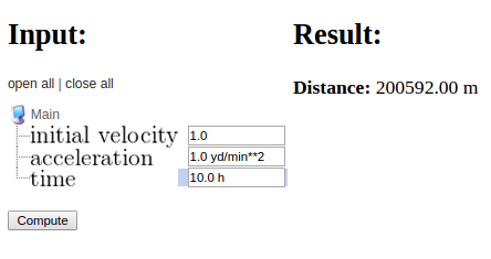
Running generate_distance_GUI.py creates a Flask-based web
interface
to our distance_unit function, see Figure 1.
The text fields in this GUI allow specification of parameters with
numbers and units, e.g., acceleration with unit yards per minute squared,
as shown in the figure. Hovering the mouse slightly to the left of
the text field causes a little black window to pop up with the registered unit
of that parameter.
1: You need to have Flask and additional packages installed.
This is easy to do with a few pip install commands,
see [5] or [6].
Figure 1: Web GUI where parameters can be specified with units.
With examples shown above, the reader should be able to make use of the
PhysicalQuantity object and the Parampool package in programs
and thereby work safely with units. For the coming text, where we discuss the
craft of scaling in detail, we shall just work in standard SI units
and avoid unit conversion so there will be no more use of
PhysicalQuantity and Parampool.