The convection-diffusion equation
Convection-diffusion without a force term
We now add a convection term \( \boldsymbol{v}\cdot\nabla u \) to the diffusion equation to obtain the well-known convection-diffusion equation: $$ \begin{equation} \frac{\partial u}{\partial t} + \v\cdot\nabla u = \dfc\nabla^2 u, \quad x,y, z\in \Omega,\ t\in (0, T]\tp \tag{3.69} \end{equation} $$ The velocity field \( \v \) is prescribed, and its characteristic size \( V \) is normally clear from the problem description. In the sketch below, we have some given flow over a bump, and \( u \) may be the concentration of some substance in the fluid. Here, \( V \) is typically \( \max_y v(y) \). The characteristic length \( L \) could be the entire domain, \( L=c+\ell \), or the height of the bump, \( L=D \). (The latter is the important length scale for the flow.)
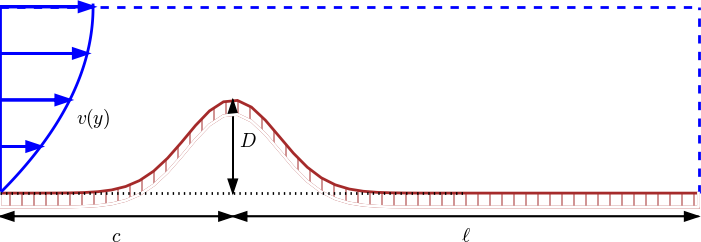
Inserting $$ \bar x = \frac{x}{x_c},\ \bar y = \frac{y}{y_c},\ \bar z = \frac{z}{z_c}, \ \bar t = \frac{t}{t_c}, \ \bar\v = \frac{\v}{V}, \ \bar u =\frac{u}{u_c}$$ in (3.69) yields $$ \frac{u_c}{t_c} \frac{\partial \bar u}{\partial \bar t} + \frac{u_c V}{L}\bar\v\cdot\bar\nabla\bar u = \frac{\dfc u_c}{L^2}\bar\nabla^2\bar u, \quad \bar x,\bar y,\bar z\in \Omega,\ \bar t\in (0,\bar T]\tp $$ For \( u_c \) we simply introduce the symbol \( U \), which we may estimate from an initial condition. It is not critical here, since it vanishes from the scaled equation anyway, as long as there is no source term present. With some velocity measure \( V \) and length measure \( L \), it is tempting to just let \( t_c = L/V \). This is the characteristic time it takes to transport a signal by convection through the domain. The alternative is to use the diffusion length scale \( t_c=L^2/\dfc \). A common physical scenario in convection-diffusion problems is that the convection term \( \v\cdot\nabla u \) dominates over the diffusion term \( \dfc\nabla^2 u \). Therefore, the time scale for convection (\( L/V \)) is most appropriate of the two. Only when the diffusion term is very much larger than the convection term (corresponding to very small Peclet numbers, see below) \( t_c=L^2/\dfc \) is the right time scale.
The non-dimensional form of the PDE with \( t_c=L/V \) becomes $$ \begin{equation} \frac{\partial \bar u}{\partial \bar t} + \bar\v\cdot\bar\nabla\bar u = \hbox{Pe}^{-1}\bar\nabla^2\bar u, \quad \bar x,\bar y,\bar z\in \Omega,\ \bar t\in (0,\bar T], \tag{3.70} \end{equation} $$ where Pe is the Peclet number, $$ \hbox{Pe} = \frac{LV}{\dfc}\tp$$ Estimating the size of the convection term \( \v\cdot\nabla u \) as \( VU/L \) and the diffusion term \( \dfc\nabla^2 u \) as \( \dfc U/L^2 \), we see that the Peclet number measures the ratio of the convection and the diffusion terms: $$ \hbox{Pe} = \frac{\hbox{convection}}{\hbox{diffusion}} = \frac{VU/L}{\dfc U/L^2}= \frac{LV}{\dfc}\tp $$
In case we use the diffusion time scale \( t_c=L^2/\dfc \), we get the non-dimensional PDE $$ \begin{equation} \frac{\partial \bar u}{\partial \bar t} + \hbox{Pe}\,\bar\v\cdot\bar\nabla\bar u = \bar\nabla^2\bar u, \quad \bar x,\bar y,\bar z\in \Omega,\ \bar t\in (0,\bar T]\tp \tag{3.71} \end{equation} $$
Discussion of scales and balance of terms in the PDE
We see that (3.70) and (3.71) are not equal, and they are based on two different time scales. For moderate Peclet numbers around 1, all terms have the same size in (3.70), i.e., a size around unity. For large Peclet numbers, (3.70) expresses a balance between the time derivative term and the convection term, both of size unity, and then there is a very small \( \hbox{Pe}^{-1}\bar\nabla^2\bar u \) term because Pe is large and \( \bar\nabla^2\bar u \) should be of size unity. That the convection term dominates over the diffusion term is consistent with the time scale \( t_c=L/V \) based on convection transport. In this case, we can neglect the diffusion term as Pe goes to infinity and work with a pure convection (or advection) equation $$ \frac{\partial \bar u}{\partial \bar t} + \bar\v\cdot\bar\nabla\bar u = 0\tp $$
For small Peclet numbers, \( \hbox{Pe}^{-1}\bar\nabla^2\bar u \) becomes very large and can only be balanced by two terms that are supposed to be unity of size. The time-derivative and/or the convection term must be much larger than unity, but that means we use suboptimal scales, since right scales imply that \( \partial\bar u/\partial\bar t \) and \( \bar v\cdot\bar\nabla\bar u \) are of order unity. Switching to a time scale based on diffusion as the dominating physical effect gives (3.71). For very small Peclet numbers this equation tells that the time-derivative balances the diffusion. The convection term \( \bar\v\cdot\bar\nabla\bar\u \) is around unity in size, but multiplied by a very small coefficient Pe, so this term is negligible in the PDE. An approximate PDE for small Peclet numbers is therefore $$ \frac{\partial \bar u}{\partial \bar t} = \bar\nabla^2\bar u\tp $$
Scaling can, with the above type of reasoning, be used to neglect terms from a differential equation under precise mathematical conditions.
Stationary PDE
Suppose the problem is stationary and that there is no need for any time scale. How is this type of convection-diffusion problem scaled? We get $$ \frac{VU}{L}\bar\v\cdot\bar\nabla\bar u = \frac{\dfc U}{L^2}\bar\nabla^2\bar u, $$ or $$ \begin{equation} \bar\v\cdot\bar\nabla\bar u = \hbox{Pe}^{-1}\bar\nabla^2\bar u\tp \tag{3.72} \end{equation} $$ This scaling only "works" for moderate Peclet numbers. For very small or very large Pe, either the convection term \( \bar\v\cdot\bar\nabla\bar u \) or the diffusion term \( \bar\nabla^2\bar u \) must deviate significantly from unity.
Consider the following 1D example to illustrate the point: \( \v = v\ii \), \( v>0 \) constant, a domain \( [0,L] \), with boundary conditions \( u(0)=0 \) and \( u(L)=U_L \). (The vector \( \ii \) is a unit vector in \( x \) direction.) The problem with dimensions is now $$ vu^{\prime} = \dfc u^{\prime\prime},\quad u(0)=0,\ u(L)=U_L\tp$$ Scaling results in $$ \frac{d\bar u}{d\bar x} = \hbox{Pe}^{-1}\frac{d^2\bar u}{d\bar x^2},\quad \bar x\in (0,1),\quad \bar u(0)=0,\ \bar u(1) = 1,$$ if we choose \( U=U_L \). The solution of the scaled problem is
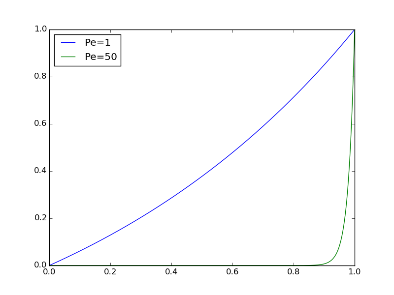
\[ \bar u(\bar x) = \frac{1 - e^{\bar x{\small\hbox{Pe}}}}{1 - e^{\small\hbox{Pe}}}\tp\] Figure 16 indicates how \( \bar u \) depends on Pe: small Pe values give approximately a straight line while large Pe values lead to a boundary layer close to \( x=1 \), where the solution changes very rapidly.
Figure 16: Solution of scaled problem for 1D convection-diffusion.
We realize that for large Pe, $$ \max_{\bar x}\frac{d\bar u}{d\bar x} \approx \hbox{Pe},\quad \max_{\bar x}\frac{d^2\bar u}{d\bar x^2} \approx \hbox{Pe}^{2},$$ which are consistent results with the PDE, since the double derivative term is multiplied by \( \hbox{Pe}^{-1} \). For small Pe, $$ \max_{\bar x}\frac{d\bar u}{d\bar x}\approx 1,\quad \max_{\bar x}\frac{d^2\bar u}{d\bar x^2} \approx 0,$$ which is also consistent with the PDE, since an almost vanishing second-order derivative is multiplied by a very large coefficient \( \hbox{Pe}^{-1} \). However, we have a problem with very large derivatives of \( \bar u \) when Pe is large.
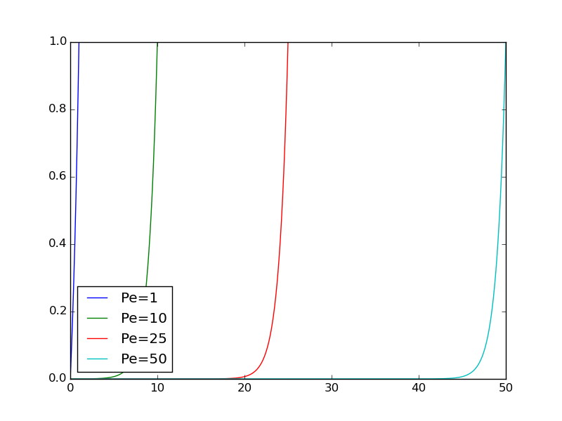
To arrive at a proper scaling for large Peclet numbers, we need to remove the Pe coefficient from the differential equation. There are only two scales at our disposals: \( u_c \) and \( x_c \) for \( u \) and \( x \), respectively. The natural value for \( u_c \) is the boundary value \( U_L \) at \( x=L \). The scaling of \( Vu_x = \dfc u_{xx} \) then results in $$ \frac{d\bar u}{d\bar x} = \frac{\dfc}{Vx_c}\frac{d^2\bar u}{d\bar x^2}, \quad \bar x\in (0,\bar L),\quad \bar u(0)=0,\ \bar u(\bar L)=1,$$ where \( \bar L = L/x_c \). Choosing the coefficient \( \dfc/(Vx_c) \) to be unity results in the scale \( x_c=\dfc/V \), and \( \bar L \) becomes Pe. The final, scaled boundary-value problem is now $$ \frac{d\bar u}{d\bar x} = \frac{d^2\bar u}{d\bar x^2}, \quad \bar x \in (0, \hbox{Pe}), \quad \bar u(0)=0,\ \bar u(\hbox{Pe})=1,$$ with solution $$ \bar u(\bar x) = \frac{1 - e^{\bar x}}{1 - e^{\small\mbox{Pe}}}\tp$$ Figure 17 displays \( \bar u \) for some Peclet numbers, and we see that the shape of the graphs are the same with this scaling. For large Peclet numbers we realize that \( \bar u \) and its derivatives are around unity (\( 1-e^{\hbox{Pe}}\approx -e^{\small\hbox{Pe}} \)), but for small Peclet numbers \( d\bar u/d\bar x \sim \hbox{Pe}^{-1} \).
Figure 17: Solution of scaled problem where the length scale depends on the Peclet number.
The conclusion is that for small Peclet numbers, \( x_c=L \) is an appropriate length scale. The scaled equation \( \hbox{Pe}\,\bar u' = \bar u'' \) indicates that \( \bar u''\approx 0 \), and the solution is close to a straight line. For large Pe values, \( x_c=\dfc/V \) is an appropriate length scale, and the scaled equation \( \bar u' = \bar u'' \) expresses that the terms \( \bar u' \) and \( \bar u'' \) are equal and of size around unity.
Convection-diffusion with a source term
Let us add a force term \( f(\x,t) \) to the convection-diffusion equation: $$ \begin{equation} \frac{\partial u}{\partial t} + \v\cdot\nabla u = \dfc\nabla^2 u + f\tp \tag{3.73} \end{equation} $$ The scaled version reads $$ \frac{\partial\bar u}{\partial\bar t} + \frac{t_cV}{L}\bar\v\cdot\bar\nabla \bar u = \frac{t_c\dfc}{L^2}\bar\nabla^2 \bar u + \frac{t_cf_c}{u_c}\bar f\tp $$ We can base \( t_c \) on convective transport: \( t_c = L/V \). Now, \( u_c \) could be chosen to make the coefficient in the source term unity: \( u_c = t_cf_c = Lf_c/V \). This leaves us with $$ \frac{\partial\bar u}{\partial\bar t} + \bar\v\cdot\bar \nabla\bar u = \hbox{Pe}^{-1}\bar \nabla^2 \bar u + \bar f\tp $$
In the diffusion limit, we base \( t_c \) on the diffusion time scale: \( t_c=L^2/\dfc \), and the coefficient of the source term set to unity determines \( u_c \) according to $$ \frac{L^2 f_c}{\dfc u_c} = 1\quad\Rightarrow\quad u_c = \frac{L^2 f_c}{\dfc}\tp$$ The corresponding PDE reads $$ \frac{\partial\bar u}{\partial\bar t} + \hbox{Pe}\,\bar\v\cdot\bar \nabla\bar u = \bar\nabla^2 \bar u + \bar f, $$ so for small Peclet numbers, which we have, the convective term can be neglected and we get a pure diffusion equation with a source term.
What if the problem is stationary? Then there is no time scale and we get $$ \frac{V u_c}{L}\bar\v\cdot\bar \nabla \bar u = \frac{u_c \dfc}{L^2}\bar\nabla^2 \bar u + f_c\bar f, $$ or $$ \bar\v\cdot\bar \nabla \bar u = \hbox{Pe}^{-1}\bar\nabla^2 \bar u + \frac{f_c L}{V u_c}\bar f\tp $$ Again, choosing \( u_c \) such that the source term coefficient is unity leads to \( u_c= f_c L/V \). Alternatively, \( u_c \) can be based on the initial condition, with similar results as found in the sections on the wave and diffusion PDEs.
Exercises
Problem 3.1: Stationary Couette flow
A fluid flows between two flat plates, with one plate at rest while the other moves with velocity \( U_0 \). This classical flow case is known as stationary Couette flow.
a) Directing the \( x \) axis in the flow direction and letting \( y \) be a coordinate perpendicular to the walls, one can assume that the velocity field simplifies to \( \u = u(y)\ii \). Show from the Navier-Stokes equations that the boundary-value problem for \( u(y) \) is $$ u^{\prime\prime}(u) = 0,\quad u(0)=0,\ u(H)=U_0\tp$$ We have here assumed at \( y=0 \) corresponds to the plate at rest and that \( y=H \) represents the plate that moves. There are no pressure gradients present in the flow.
b) Scale the problem in a) and show that the result has no physical parameters left in the model: $$ \frac{d^2\bar u}{d\bar y^2} = 0,\quad \bar u(0)=0,\ \bar u(1)=1\tp$$
c) We can compute \( \bar u(\bar y) \) from one numerical simulation (or a straightforward integration of the differential equation). Set up the formula that finds \( u(y; H, u_0) \) from \( \bar u(\bar y) \) for any values of \( H \) and \( U_0 \).
Filename: stationary_Couette.
Remarks
The problem for \( u \) is a classical two-point boundary-value problem in applied mathematics and arises in a number of applications, where Couette flow is just one example. Heat conduction is another example: \( u \) is temperature, and the heat conduction equation for an insulated rod reduces to \( u^{\prime\prime}=0 \) under stationary conditions and no heat source. Controlling the end \( x=0 \) at 0 degrees Celsius the other end \( x=L \) at \( U_0 \) degrees Celsius, gives the same boundary conditions as in the above flow problem. The scaled problem is of course the same whether we have flow of fluid or heat.
Exercise 3.2: Couette-Poiseuille flow
Viscous fluid flow between two infinite flat plates \( z=0 \) and \( z=H \) is governed by $$ \begin{align} \mu u''(z) &= -\beta \tag{3.74}\\ u(0) &= 0, \tag{3.75}\\ u(H) &= U_0\tp \tag{3.76} \end{align} $$ Here, \( u(z) \) is the fluid velocity in \( x \) direction (perpendicular to the \( z \) axis), \( \mu \) is the dynamic viscosity of the fluid, \( \beta \) is a positive constant pressure gradient, and \( U_0 \) is the constant velocity of the upper plate \( z=H \) in \( x \) direction. The model represents Couette flow for \( \beta=0 \) and Poiseuille flow for \( U_0=0 \).
a) Find the exact solution \( u(z) \). Point out how \( \beta \) and \( U_0 \) influence the magnitude of \( u \).
SymPy can integrate the differential equation twice and fit the integration constants to the boundary conditions:
import sympy as sym
mu, beta, z, H = sym.symbols('mu beta z H',
                             real=True, positive=True)
U0, C1, C2 = sym.symbols('U0 C1 C2', real=True)

# Integrate u''(z) = -beta/mu twice and add integration constants
u = sym.integrate(sym.integrate(-beta/mu, z) + C1, z) + C2

# Use the boundary conditions
eq = [sym.Eq(u.subs(z, 0), 0),
      sym.Eq(u.subs(z, H), U0)]
s = sym.solve(eq, [C1, C2])
print s
u = u.subs(C1, s[C1]).subs(C2, s[C2])
u = sym.simplify(sym.expand(u))
The result becomes $$ u(z) = \frac{z}{2 H \mu} \left(H \beta \left(H - z\right) + 2 U_{0} \mu\right)\tp $$
The maximum value of \( u \) is found by
# Find max u
dudz = sym.diff(u, z)
s = sym.solve(dudz, z)
print s
umax = u.subs(z, s[0])
umax = sym.simplify(sym.expand(umax))
and reads $$ \max_z u = \frac{H^{2} \beta}{8 \mu} + \frac{U_{0}}{2} + \frac{U_{0}^{2} \mu}{2 H^{2} \beta}\tp $$ If the pressure gradient is the dominating driving force, we can neglect the \( U_0 \) terms: \( \max_z u = H^2\beta/(8\mu) \). In case the movement of the upper plate is much more important than the pressure gradient for driving the flow, we can neglect the \( \beta \) terms. However, we must then resort to the \( u(z) \) expression for \( \beta=0 \), \( u(z)=zU_0/H \), and realize that the maximum then is obtained at the boundary for \( z=H \): \( \max_z h=U_0 \) (as intuitively obvious).
b) Scale the problem.
Introducing $$ \bar z = \frac{z}{z_c}, \quad \bar u (\bar z) = \frac{u(z_c\bar z)}{u_c},$$ in the equation gives $$ \frac{d^2\bar u}{d\bar z^2} = -\frac{z_c^2\beta}{\mu u_c}\tp$$ The natural scale for \( z_c \) is \( H \) since that makes \( \bar z\in [0,1] \). For the two terms in the differential equation to be of order unity (with a correct scaling, the left-hand side should be of order unity), we must have $$ u_c = \frac{H^2\beta}{\mu}\tp$$ The boundary value problem is $$ \begin{align*} \frac{d^2\bar u}{d\bar z^2} &= -1,\quad &\bar z\in (0,1),\\ \bar u(0) &= 0,\\ \bar u(1) &= \alpha, \end{align*} $$ where \( \alpha \) is a dimensionless number $$ \alpha = \frac{\mu U_0}{H^2\beta}\tp$$ This is meaningful only for \( \beta\neq 0 \).
Looking at the exact solution, we see that \( \max_z u = H^2\beta/(8\mu) \), and with this \( \max_z u \) as \( u_c \) we get a differential equation \( \bar u'' = -8 \) instead, and \( \bar u\in [0,1] \) (if \( U_0=0 \)). However, the factor \( 1 \) or \( 8 \) on the right-hand side is not significant, neither if \( \bar u\in [0,1] \) or \( \bar u\in [0,8] \).
The scale \( u_c \) used above is relevant if the pressure gradient is the dominating force. If \( U_0 \) is more important than \( \beta \), or \( \beta =0 \), we choose \( u_c=U_0 \) and get instead $$ \begin{alignat}{2} \frac{d^2\bar u}{d\bar z^2} &= -\alpha^{-1},\quad &\bar z\in (0,1),\\ \bar u(0) &= 0,\\ \bar u(1) &= 1\tp \end{alignat} $$
Filename: Couette_wpressure.
Exercise 3.3: Pulsatile pipeflow
The flow of a viscous fluid in a straight pipe with circular cross section with radius \( R \) is governed by $$ \begin{alignat}{2} \varrho\frac{\partial u}{\partial t} &= \frac{\mu}{r}\frac{\partial}{\partial r} \left(r\frac{\partial u}{\partial r}\right) - P(t), & r\in (0,R),\ t\in (0,T],\\ \frac{\partial u}{\partial r}(0,t) &= 0, & t\in (0,T],\\ u(R,t) &= 0, & t\in (0,T],\\ u(r,0) &= 0, & r\in [0,R]. \end{alignat} $$ The quantity \( u(r,t) \) is the fluid velocity, \( P(t) \) is a given pressure gradient, \( \varrho \) is the fluid density, and \( \mu \) is the dynamic viscosity.
Assume \( P(t) = A\cos\omega t \). Scale the problem and identify appropriate dimensionless numbers. Thereafter, assume \( P(t) \) is a more complicated function, but still period with period \( p \). Discuss how the scaling can be extended to this case.
We introduce dimensionless quantities: $$ \bar r = \frac{r}{R},\quad \bar t = \frac{t}{t_c},\quad \bar u = \frac{u}{u_c}\tp$$ The function \( P(t) \) can be scaled as $$ \bar P(\bar t) = \frac{P(t_c\bar t)}{A} = \sin (t_c\omega \bar t)\tp$$ Inserted in the PDE, we get $$ \frac{\partial\bar u}{\partial\bar t} = \frac{t_c \nu }{R^2}\frac{1}{\bar r}\frac{\partial}{\partial\bar r} \left(\bar r\frac{\partial\bar u}{\partial\bar r}\right) - \frac{t_c A}{\varrho u_c}\sin (t_c\omega\bar t),$$ where \( \mu = \mu/\varrho \).
The scale for \( u \) can be explored by seeking an analytical solution of the problem. Such solutions do exist, they are typically series expansions of Bessel functions, and it is not so easy to extract a simple expression for the maximum value of \( |u(r,t)| \). A simpler approach is to estimate \( u_c \) by demanding the coefficient in the pressure term to be of unit size: $$ u_c = \frac{t_cA}{\varrho}\tp$$ There are two choices of time scales: the pressure time scale \( t_c=1/\omega \) and the viscosity (or diffusion) time scale \( t_c=R^2/nu \). With the latter, we get \( u_c = R^2 A/\mu \) and $$ \frac{\partial\bar u}{\partial\bar t} = \frac{1}{\bar r}\frac{\partial}{\partial\bar r} \left(\bar r\frac{\partial\bar u}{\partial\bar r}\right) - \sin (\alpha\bar t),$$ where $$ \alpha = \frac{R^2\omega}{\nu} = \frac{R^2/\nu}{1/\omega},$$ showing that \( \alpha \) is the ratio of the viscosity time scale and the pressure oscillation time scale.
With the pressure time scale we have $$ u_c = \frac{\varrho A}{\omega},$$ and the scaled PDE becomes $$ \frac{\partial\bar u}{\partial\bar t} = \alpha^{-1}\frac{1}{\bar r}\frac{\partial}{\partial\bar r} \left(\bar r\frac{\partial\bar u}{\partial\bar r}\right) - \sin (\bar t)\tp$$ In both cases the scaled boundary conditions become $$ \frac{\partial\bar u}{\partial\bar t} = 0,\quad \bar u(1,\bar t) = 0,$$ for \( t\in (0,T/t_c] \), and \( \bar u(\bar r, 0)=0 \) for \( \bar r\in [0,1] \).
If \( P(t) \) is not sinusoidal but periodic with period \( p \), we have that \( P \) is a function of \( \omega t \) as above, with \( \omega = 2\pi/p \). Everything in the scaling remains the same, just the \( \sin \) term changes to \( P(\alpha\bar t) \) if the time scale is based on viscosity (diffusion), and \( P(\bar t) \) if the time scale is based on the pressure oscillations.
Filename: pipeflow.
Exercise 3.4: The linear cable equation
A key PDE in neuroscience is the cable equation, here given in its simplest linear form: $$ \begin{equation} \tau\frac{\partial u}{\partial t} = \lambda^2\frac{\partial^2 u}{\partial x^2} -u\tp \tag{3.77} \end{equation} $$ The unknown \( u \) is the voltage (measured in volt) associated with an electric current along one-dimensional dendrites ("cables") in neural networks, while \( \tau \) and \( \lambda \) are given parameters.
Scale (3.77) in three ways: 1) let all terms in the scaled equation have unit coefficients, 2) use the domain size \( L \) as spatial scale and base the time scale on diffusion, 3) use the domain size \( L \) as spatial scale and base the time scale on reaction, i.e., the \( -u \) term.
Straightforward scaling, with scales \( u_c \), \( t_c \), and \( x_c \), leads in the first step to $$ \frac{\partial\bar u}{\partial\bar t} = \frac{t_c\lambda^2}{\tau x_c^2}\frac{\partial^2\bar u}{\partial\bar x^2} - \frac{t_c}{\tau}\bar u\tp$$ Assuming that all terms are equally important and of unit size in the scaled PDE, we get a uniquely determined length and space scale: $$ t_c = \tau,\quad x_c = \lambda\tp$$ The scaled cable equation is then $$ \frac{\partial\bar u}{\partial\bar t} = \frac{\partial^2\bar u}{\partial\bar x^2} - \bar u\tp $$
Let now the spatial scale be fixed as \( x_c=L \). Basing \( t_c \) on diffusion means \( t_c = \tau (L/\lambda)^2 \), and the scaled PDE becomes $$ \frac{\partial\bar u}{\partial\bar t} = \frac{\partial^2\bar u}{\partial\bar x^2} - \beta\bar u,$$ where $$ \beta = \left(\frac{L}{\lambda}\right)^2\tp$$
Basing \( t_c \) on the reaction scale, i.e., the balance of the time derivative and the reaction term, gives \( t_c=\tau \) and the scaled PDE $$ \frac{\partial\bar u}{\partial\bar t} = \beta^{-1}\frac{\partial^2\bar u}{\partial\bar x^2} - \bar u\tp$$
In neuroscience applications of the cable equation to dendrites, it appears that \( \lambda \) is about 1 mm and of the same order of magnitude as the cable length, so \( \beta \) is around 1 in size. Then there are not big differences in these scalings, and the first one is to be preferred. The two others are more suitable when \( \beta \) is small or large, e.g., such that the term with \( \beta \) can be left out of the PDE.
Filename: cable_eq.
Exercise 3.5: Heat conduction with discontinuous initial condition
Two pieces of metal at different temperature are brought in contact at \( t=0 \). The following initial-boundary value problem governs the temperature evolution in the two pieces: $$ \begin{alignat}{2} \frac{\partial u}{\partial t} &= \dfc\nabla^2 u,\ & \x\in\Omega,\ t\in (0,T],\\ u(\x,0)&=I(x), & \x\in \Omega, \tag{3.78}\\ -\dfc\frac{\partial u}{\partial n} &= h(u-u_S), & x\in\partial\Omega,\ t\in (0,T]. \tag{3.79} \end{alignat} $$ Here, \( u(\x,t) \) is the temperature, \( \dfc \) the effective heat diffusion coefficient (assuming both pieces are homogeneous and of the same type of metal), and \( u_S \) is the surrounding temperature. The domain \( \Omega \) consists of the two pieces \( \Omega_1 \) and \( \Omega_2 \): \( \Omega = \Omega_1\cup\Omega_2 \). The initial condition can be specified as $$ I(x) = \left\lbrace\begin{array}{ll} U_1, & \x\in\Omega_1,\\ U_2, & \x\in\Omega_2, \end{array}\right. $$ where \( U_1 \) and \( U_2 \) are the constant initial temperatures in each piece.
Thinking of two identical pieces \( \Omega_1 \) and \( \Omega_2 \) with shapes as bricks, it is tempting to develop a one-dimensional model, especially if the pieces are somewhat slender. We then expect the main temperature variations to take place in the \( x \) direction, where the \( x \) axis is perpendicular to the contact surface between the pieces. A simplified PDE problem, neglecting variations in the \( y \) and \( z \) directions, takes the form $$ \begin{alignat}{2} \frac{\partial v}{\partial t} &= \dfc \frac{\partial^2 v}{\partial x^2} -\frac{hP}{A}(v(x,t) -u_S),\ & x\in (0,L),\ t\in (0,T], \tag{3.80}\\ v(x,0)&=I(x), & x\in (0,L),\\ \dfc\frac{\partial v}{\partial x} &= h(v(x,t)-u_S), & x=0,\ t\in (0,T], \tag{3.81}\\ -\dfc\frac{\partial v}{\partial x} &= h(v(x,t)-u_S), & x=L,\ t\in (0,T], \tag{3.82} \end{alignat} $$ with $$ I(x) = \left\lbrace\begin{array}{ll} U_1, & x\in [0,L/2),\\ U_2, & x\in [L/2, L]\tp \end{array}\right. $$ The parameter \( P \) is the perimeter of the cross section and \( A \) is the area of the cross section. Scale this problem.
We expect the temperature to start from the discontinuous state with \( U_1 \) and \( U_2 \) and approach the surrounding temperature \( u_S \) in the cooling law as \( t\rightarrow\infty \). One suitable scaling is then $$ \bar v = \frac{v - \min (U_1,U_2)}{u_S-\min (U_1, U_2)},$$ since this implies that \( u \) varies from 0 to 1. Without loss of generality we number the bricks such that \( U_1 < U_2 \), so $$ \bar v = \frac{v - U_1}{u_S-U_1}\tp$$ Furthermore, $$ \bar x = \frac{x}{L},\quad \bar t = \frac{t}{t_c}\tp$$ Inserted in the governing PDE, we have $$ \frac{\partial\bar v}{\partial\bar t} = \frac{t_c\dfc}{L^2}\frac{\partial^2\bar v}{\partial\bar x^2} -\frac{t_c hP}{A(u_S-U_1)} (U_1 + (u_S-U_1) \bar v(x,t) - u_S),$$ which simplifies to $$ \frac{\partial\bar v}{\partial\bar t} = \frac{t_c\dfc}{L^2}\frac{\partial^2\bar v}{\partial\bar x^2} -\frac{t_c hP}{A} (\bar v(x,t) - 1)\tp$$ The natural time scale is that of diffusion: \( t_c = L^2/\dfc \). This choice results in the scaled PDE $$ \frac{\partial\bar v}{\partial\bar t} = \frac{\partial^2\bar v}{\partial\bar x^2} -\overline{\hbox{Bi}}^{}\,(\bar v(x,t) - 1),$$ where the dimensionless number $$ \overline{\hbox{Bi}}^{} = \frac{hL^2P}{\dfc A}$$ can be interpreted as a modified Biot number (if \( A/P=L \), it would an ordinary Biot number, but here this is not an appropriate approximation: for bricks with square cross section of length \( a \), \( A/P=a/4 \), and for a circular cross section, \( A/P=R/2 \)). This modified Biot number governs the significance of lateral heat loss/gain to/from the environment.
The scaled initial condition becomes $$ \bar v(\bar x,0)=0 \hbox{ if } 0\leq x < 1/2\hbox{ else } \beta,$$ where \( \beta \) is the dimensionless number $$ \beta = \frac{U_2 - U_1}{U_s - U_1}\tp$$ The scaled boundary conditions take the form $$ \frac{\partial}{\partial\bar x}\bar v(0,t) = \hbox{Bi}\, (\bar v(0,t)-1),\quad -\frac{\partial}{\partial\bar x}\bar v(L,t) = \hbox{Bi}\, (\bar v(L,t)-1), $$ where Bi is the standard Biot number for heat conduction from solids: $$ \hbox{Bi} = \frac{Lh}{\dfc}\tp$$
Here is a simulation with \( \hbox{Bi}=0.01 \), \( \overline{\hbox{Bi}}^{} = 0.2 \),
and \( \beta =1.5 \)
(using the diffusion_two_metal_pieces function in
session.py).
Another temperature scaling is also possible: $$ \bar v = \frac{v - U_s}{U_2-U_s}\tp$$ The initial condition is then $$ \bar v(\bar x,0)=\gamma \hbox{ if } 0\leq x < 1/2\hbox{ else } 1,$$ where \( \gamma \) is the dimensionless number $$ \gamma = \frac{U_1 - U_s}{U_2 - U_s}\tp$$ Note that \( \gamma < 1 \) if \( U_1 < U_2 \), and we expect \( \bar v\in [0, 1] \) (\( \bar v\rightarrow 0 \) as \( \bar t\rightarrow\infty \)). The PDE now becomes homogeneous, $$ \frac{\partial\bar v}{\partial\bar t} = \frac{\partial^2\bar v}{\partial\bar x^2} -\overline{\hbox{Bi}}^{}\,\bar v(x,t),$$ and the boundary conditions take the form $$ \frac{\partial}{\partial\bar x}\bar v(0,t) = \hbox{Bi}\, \bar v(0,t),\quad -\frac{\partial}{\partial\bar x}\bar v(L,t) = \hbox{Bi}\, \bar v(L,t)\tp $$ Many will find the homogeneous PDE and boundary conditions of the latter scaling attractive, especially for analytical solution of the problem.
Filename: metal_pieces.
Remarks
We can derive (3.80)-(3.82) from (3.78)-(3.79). The idea is to integrate the governing PDE (3.80) in the two directions where we expect negligible variations, use the Gauss divergence theorem in these directions, and apply the cooling boundary condition. Let \( A \) be the cross section of the bricks. Integrating over \( A \) gives $$ \begin{align*} \int\limits_A \frac{\partial u}{\partial t}dydz &= \int\limits_A \dfc\left( \frac{\partial^2 u}{\partial x^2} + \frac{\partial^2 u}{\partial y^2} + \frac{\partial^2 u}{\partial z^2} \right)dydz \\ &=\int\limits_A \dfc \frac{\partial^2 u}{\partial x^2} dydz + \int\limits_A \dfc\left( \frac{\partial^2 u}{\partial y^2} + \frac{\partial^2 u}{\partial z^2} \right)dydz \\ & = \int\limits_A \dfc \frac{\partial^2 u}{\partial x^2} dydz + \dfc\int\limits_{\partial A}\frac{\partial u}{\partial n}ds\\ & = \int\limits_A \dfc \frac{\partial^2 u}{\partial x^2} dydz -h(v(x,t) -u_S)P\tp \end{align*} $$ The parameter \( P \) is the perimeter of the cross section \( A \). The function \( v(x,t) \) means \( u(\x,t) \) evaluated at the boundary \( \partial A \). Assuming \( u \) to vary little across the cross section \( A \), we can approximate the integrals by \( u \) evaluated at \( \partial A \) as \( v \): $$ \int\limits_A \frac{\partial u}{\partial t}dydz\approx A \frac{\partial}{\partial t} v(x,t), \quad \int\limits_A \dfc \frac{\partial^2 u}{\partial x^2} dydz \approx A \dfc \frac{\partial^2 v}{\partial x^2}, $$ where \( A \) now is the cross-section area. The result is the 1D initial-boundary value problem (3.80)-(3.82).
Problem 3.6: Scaling a welding problem
Welding equipment makes a very localized heat source that moves in time. We shall investigate the heating due to welding and choose, for maximum simplicity, a one-dimensional heat equation with a fixed temperature at the ends (a 2D or 3D model with cooling conditions at the boundaries would be of greater physical significance, but now the scaling is in focus). The effect of melting is not included in the heat equation. Our goal is to investigate alternative scalings through numerical experimentation.
The governing PDE problem reads $$ \begin{alignat*}{2} \varrho c\frac{\partial u}{\partial t} &= k\frac{\partial^2 u}{\partial x^2} + f, & x\in (0,L),\ t\in (0,T),\\ u(x,0) &= U_s, & x\in [0,L],\\ u(0,t) = u(L,t) &= U_s, & t\in (0,T]. \end{alignat*} $$ Here, \( u \) is the temperature, \( \varrho \) the density of the material, \( c \) a heat capacity, \( k \) the heat conduction coefficient, \( f \) is the heat source from the welding equipment, and \( U_s \) is the initial constant (room) temperature in the material.
The boundary conditions at \( x=0,L \) are set for convenience – some sort of heat flux out of the boundary, modeled in terms of a cooling condition \( -ku_x = h(u-U_s) \), for a heat transfer coefficient \( h \), would yield a more physically relevant model. Also, only a full 3D geometry with such heat loss at the boundary is physically relevant, as neglecting a space dimension means insulated boundaries perpendicular to this direction. However, since the focus is on scaling, we prefer to work with the simplest possible model, which is one-dimensional, has Dirichlet boundary conditions, and neglects melting. The latter effect is very local and just stalls the temperature field locally – it does not affect the transport of heat away from the welding source in a significant way.
A possible model for the heat source is a moving Gaussian function: $$ f = A\exp{\left(-\frac{1}{2}\left(\frac{x-vt}{\sigma}\right)^2\right)},$$ where \( A \) is the strength, \( \sigma \) is a parameter governing how peak-shaped (or localized in space) the heat source is, and \( v \) is the velocity (in positive \( x \) direction) of the source.
a) Let \( x_c \), \( t_c \), \( u_c \), and \( f_c \) be scales, i.e., characteristic sizes, of \( x \), \( t \), \( u \), and \( f \), respectively. The natural choice of \( x_c \) and \( f_c \) is \( L \) and \( A \), since these make the scaled \( x \) and \( f \) in the interval \( [0,1] \). If each of the three terms in the PDE are equally important, we can find \( t_c \) and \( u_c \) by demanding that the coefficients in the scaled PDE are all equal to unity. Perform this scaling. Use scaled quantities in the arguments for the exponential function in \( f \) too and show that $$ \bar f= \exp{(-\frac{1}{2}\beta^2(\bar x -\gamma \bar t)^2)},$$ where \( \beta \) and \( \gamma \) are dimensionless numbers. Give an interpretation of \( \beta \) and \( \gamma \).
We introduce $$ \bar x=\frac{x}{L},\quad \bar t = \frac{t}{t_c},\quad \bar u = \frac{u-U_s}{u_c}, \quad \bar f=\frac{f}{A}\tp$$ Inserted in the PDE and dividing by \( \varrho c u_c/t_c \) such that the coefficient in front of \( \partial\bar u/\partial\bar t \) becomes unity, and thereby all terms become dimensionless, we get $$ \frac{\partial\bar u}{\partial\bar t} = \frac{k t_c}{\varrho c L^2}\frac{\partial^2\bar u}{\partial\bar x^2} + \frac{A t_c}{\varrho c u_c}\bar f\tp $$ Demanding that all three terms are equally important, it follows that $$ \frac{k t_c}{\varrho c L^2} = 1,\quad \frac{A t_c}{\varrho c u_c}=1\tp$$ These constraints imply the diffusion time scale $$ t_c = \frac{\varrho cL^2}{k},$$ and a scale for \( u_c \), $$ u_c = \frac{AL^2}{k}\tp$$ The scaled PDE reads $$ \frac{\partial\bar u}{\partial\bar t} = \frac{\partial^2\bar u}{\partial\bar x^2} + \bar f\tp$$
Scaling \( f \) results in $$ \begin{align*} \bar f &= \exp{\left(-\frac{1}{2}\left(\frac{x-vt}{\sigma}\right)^2\right)}\\ &= \exp{\left(-\frac{1}{2}\frac{L^2}{\sigma^2} \left(\bar x- \frac{vt_c}{L}\bar t\right)^2\right)}\\ &= \exp{\left(-\frac{1}{2}\beta^2\left(\bar x-\gamma \bar t\right)^2\right)}, \end{align*} $$ where \( \beta \) and \( \gamma \) are dimensionless numbers: $$ \beta = \frac{L}{\sigma},\quad \gamma = \frac{vt_c}{L} = \frac{v\varrho cL}{k}\tp$$ The \( \sigma \) parameter measures the width of the Gaussian peak, so \( \beta \) is the ratio of the domain and the width of the heat source (large \( \beta \) implies a very peak-formed heat source). The \( \gamma \) parameter arises from \( t_c/(L/v) \), which is the ratio of the diffusion time scale and the time it takes for the heat source to travel through the domain. Equivalently, we can multiply by \( t_c/t_c \) to get \( \gamma = v/(t_cL) \) as the ratio between the velocity of the heat source and the diffusion velocity.
b) Argue that at least for large \( \gamma \) we should base the time scale on the movement of the heat source. Using \( L \) as length scale, show that this gives rise to the scaled PDE $$ \frac{\partial\bar u}{\partial\bar t} = \gamma^{-1}\frac{\partial^2\bar u}{\partial\bar x^2} + \bar f, $$ and $$ \bar f = \exp{(-\frac{1}{2}\beta^2(\bar x - \bar t)^2)}\tp$$ Discuss when the scalings in a) and b) are appropriate.
We perform the scaling as in a), but this time we determine \( t_c \) such that the heat source moves with unit velocity. This means that $$ \frac{vt_c}{L} = 1\quad\Rightarrow\quad t_c = \frac{L}{v}\tp$$ Scaling of the PDE gives, as before, $$ \frac{\partial\bar u}{\partial\bar t} = \frac{k t_c}{\varrho c L^2}\frac{\partial^2\bar u}{\partial\bar x^2} + \frac{A t_c}{\varrho c u_c}\bar f\tp $$ Inserting the expression for \( t_c \), we have $$ \frac{\partial\bar u}{\partial\bar t} = \frac{k L}{\varrho c L^2v}\frac{\partial^2\bar u}{\partial\bar x^2} + \frac{A L}{v\varrho c u_c}\bar f\tp $$ We recognize the first coefficient as \( \gamma^{-1} \), while \( u_c \) can be determined from demanding the second coefficient to be unity: $$ u_c = \frac{AL}{v\varrho c}\tp$$ The scaled PDE is therefore $$ \frac{\partial\bar u}{\partial\bar t} = \gamma^{-1}\frac{\partial^2\bar u}{\partial\bar x^2} + \bar f\tp$$ If the heat source moves very fast, there is little time for the diffusion to transport the heat away from the source, and the heat conduction term becomes insignificant. This is reflected in the coefficient \( \gamma^{-1} \), which is small when \( \gamma \), the ratio of the heat source velocity and the diffusion velocity, is large.
The scaling in a) is therefore appropriate if diffusion is a significant process, i.e., the welding equipment moves at a slow speed so heat can efficiently spread out by diffusion. For large \( \gamma \), the scaling in b) is appropriate, and \( t=1 \) corresponds to having the heat source traveled through the domain (with the scaling in a), the heat source will leave the domain in short time).
c) For fast movement of the welding equipment, i.e., when heat transfer is less important than the local heating by the equipment, the typical length scale of the local heating is the size of the source, reflected by the \( \sigma \) parameter. Modify the scaling in b) when \( \sigma \) is chosen as length scale.
With \( \sigma \) as length scale, the scaled PDE has the initial form $$ \frac{\partial\bar u}{\partial\bar t} = \frac{k t_c}{\varrho c \sigma^2}\frac{\partial^2\bar u}{\partial\bar x^2} + \frac{A t_c}{\varrho c u_c}\bar f\tp $$ The scaling of \( f \) becomes $$ \begin{align*} \bar f &= \exp{\left(-\frac{1}{2}\left(\frac{x-vt}{\sigma}\right)^2\right)}\\ &= \exp{\left(-\frac{1}{2} \left(\bar x- \frac{vt_c}{\sigma}\bar t\right)^2\right)}\\ &= \exp{\left(-\frac{1}{2}\left(\bar x- \bar t\right)^2\right)}, \end{align*} $$ where we have chosen \( t_c \) as \( \sigma/v \). Inserting \( t_c \) in the PDE leads to a coefficient $$ \frac{k}{v\varrho c \sigma} = \gamma^{-1}\beta\tp$$ As before, we chose \( u_c \) to make the other coefficient equal unity, modulo a scaling factor. We then obtain \( u_c=t_c A/\rho c \), which may be read as the time each point feels the source times source strength divided to the volumetric heat capacity that includes the density. The \( \gamma^{-1}\beta \) parameter is the ratio of the moving heat source time scale \( v/\sigma \) and the diffusion time scale \( \sigma^2/(k/\varrho c) \).
The equations are as in), except that \( \beta =1 \) and \( \epsilon \) replaces \( \gamma \). Moreover, the length of the domain is now \( L/\sigma \), i.e., \( \beta \) enters the problem in the domain size.
d) A fourth kind of possible scaling is to say that for small \( \gamma \), the problem is quasi-stationary and the heat transfer balances the heat source. Determine \( u_c \) from this assumption. Use \( L \) as length scale and a time scale as in b), i.e., based on the movement of the welding equipment.
We insert the dimensionless quantities in the PDE, but this time we make the factor in the source term unity: $$ \frac{\varrho c u_c}{A t_c} \frac{\partial\bar u}{\partial\bar t} = \frac{ku_c}{AL^2}\frac{\partial^2\bar u}{\partial\bar x^2} + \bar f\tp $$ Assuming the two terms on the right-hand side balance, we must have \( ku_c/(AL^2)=1 \) and hence \( u_c= L^2A/k \). This gives the coefficient \( \varrho cL^2/(kt_c) \) on the left-hand side. From b) we have that a time scale based the movement of the heat source: \( t_c=L/v \). Now the scaled PDE becomes $$ \gamma \frac{\partial\bar u}{\partial\bar t} = \frac{\partial^2\bar u}{\partial\bar x^2} + \bar f\tp$$ The scaling of \( f \) becomes identical to the one in b).
e) One aim with scaling is to get a solution that lies in the interval \( [-1,1] \). This is not always the case when \( u_c \) is based on a scale involving a source term, as we do in a)-c). However, from the scaled PDE we realize that if we replace \( \bar f \) with \( \delta\bar f \), where \( \delta \) is a dimensionless factor, this corresponds to replacing \( u_c \) by \( u_c/\delta \). So, if we observe that \( \bar u\sim1/\delta \) in simulations, we can just replace \( \bar f \) by \( \delta \bar f \) in the scaled PDE.
Use this trick and implement the four scaled models in a)-d). Reuse
some software for the 1D diffusion equation. Make a function
run(gamma, beta=10, delta=40, scaling=1, animate=False) that runs an
implementation of the unscaled model with the given \( \gamma \), \( \beta \),
and \( \delta \) parameters as well as an indicator scaling that is 'a',
'b', and so forth. The
last argument can be used to turn screen animations on or off.
Perform experiments to find the proper value of \( \delta \) for each \( \gamma \) and for each scaling.
Equip the run function with visualization, both animation of \( \bar u \)
and \( \bar f \), and plots with \( \bar u \) and \( \bar f \) for \( t=0.2 \) and \( t=0.5 \).
Since the amplitudes of \( \bar u \) and \( \bar f \) differs by a factor \( \delta \), it is attractive to plot \( \bar f/\delta \) together with \( \bar u \).
Here is a possible general solver function for solving the 1D
diffusion equation
$$ \frac{\partial u}{\partial t} = \frac{\partial}{\partial x}
\left(\dfc(x)\frac{\partial u}{\partial x}\right) + f,$$
by the \( \theta \)-rule in time and centered finite
differences in space. The \( \theta \)-rule in time is actually just a notational
convenience that gives Forward Euler explicit time stepping for
\( \theta=0 \), Backward Euler implicit time stepping for \( \theta=0 \), and
a centered implicit Crank-Nicolson scheme for \( \theta=\half \).
The boundary conditions is of Dirichlet type: \( u(0,t)=U_L(t) \) and
\( u(L,t)=U_R(t) \).
import numpy as np
import scipy.sparse
import scipy.sparse.linalg
import time, sys


def solver(I, a, f, L, Nx, D, T, theta=0.5, u_L=1, u_R=0,
           user_action=None):
    """
    The a variable is an array of length Nx+1 holding the values of
    a(x) at the mesh points.

    Method: (implicit) theta-rule in time.

    Nx is the total number of mesh cells; mesh points are numbered
    from 0 to Nx.
    D = dt/dx**2 and implicitly specifies the time step.
    T is the stop time for the simulation.
    I is a function of x.

    user_action is a function of (u, x, t, n) where the calling code
    can add visualization, error computations, data analysis,
    store solutions, etc.
    """
    import time
    t0 = time.clock()

    x = np.linspace(0, L, Nx+1)   # mesh points in space
    dx = x[1] - x[0]
    dt = D*dx**2
    #print 'dt=%g' % dt
    Nt = int(round(T/float(dt)))
    t = np.linspace(0, T, Nt+1)   # mesh points in time

    if isinstance(a, (float,int)):
        a = np.zeros(Nx+1) + a
    if isinstance(u_L, (float,int)):
        u_L_ = float(u_L)  # must take copy of u_L number
        u_L = lambda t: u_L_
    if isinstance(u_R, (float,int)):
        u_R_ = float(u_R)  # must take copy of u_R number
        u_R = lambda t: u_R_

    u   = np.zeros(Nx+1)   # solution array at t[n+1]
    u_1 = np.zeros(Nx+1)   # solution at t[n]

    """
    Basic formula in the scheme:

    0.5*(a[i+1] + a[i])*(u[i+1] - u[i]) -
    0.5*(a[i] + a[i-1])*(u[i] - u[i-1])

    0.5*(a[i+1] + a[i])*u[i+1]
    0.5*(a[i] + a[i-1])*u[i-1]
    -0.5*(a[i+1] + 2*a[i] + a[i-1])*u[i]
    """
    Dl = 0.5*D*theta
    Dr = 0.5*D*(1-theta)

    # Representation of sparse matrix and right-hand side
    diagonal = np.zeros(Nx+1)
    lower    = np.zeros(Nx)
    upper    = np.zeros(Nx)
    b        = np.zeros(Nx+1)

    # Precompute sparse matrix (scipy format)
    diagonal[1:-1] = 1 + Dl*(a[2:] + 2*a[1:-1] + a[:-2])
    lower[:-1] = -Dl*(a[1:-1] + a[:-2])
    upper[1:]  = -Dl*(a[2:] + a[1:-1])
    # Insert boundary conditions
    diagonal[0] = 1
    upper[0] = 0
    diagonal[Nx] = 1
    lower[-1] = 0

    A = scipy.sparse.diags(
        diagonals=[diagonal, lower, upper],
        offsets=[0, -1, 1],
        shape=(Nx+1, Nx+1),
        format='csr')
    #print A.todense()

    # Set initial condition
    for i in range(0,Nx+1):
        u_1[i] = I(x[i])

    if user_action is not None:
        user_action(u_1, x, t, 0)

    # Time loop
    for n in range(0, Nt):
        b[1:-1] = u_1[1:-1] + Dr*(
            (a[2:] + a[1:-1])*(u_1[2:] - u_1[1:-1]) -
            (a[1:-1] + a[0:-2])*(u_1[1:-1] - u_1[:-2])) + \
            dt*theta*f(x[1:-1], t[n+1]) + \
            dt*(1-theta)*f(x[1:-1], t[n])
        # Boundary conditions
        b[0]  = u_L(t[n+1])
        b[-1] = u_R(t[n+1])
        # Solve
        u[:] = scipy.sparse.linalg.spsolve(A, b)

        if user_action is not None:
            user_action(u, x, t, n+1)

        # Switch variables before next step
        u_1, u = u, u_1

    t1 = time.clock()
    return t1-t0
And here is our run function tailored to the problem:
def run(gamma, beta=10, delta=40, scaling=1, animate=False):
    """Run the scaled model for welding."""
    gamma = float(gamma)  # avoid integer division
    if scaling == 'a':
        v = gamma
        a = 1
        L = 1.0
        b = 0.5*beta**2
    elif scaling == 'b':
        v = 1
        a = 1.0/gamma
        L = 1.0
        b = 0.5*beta**2
    elif scaling == 'c':
        v = 1
        a = beta/gamma
        L = beta
        b = 0.5
    elif scaling == 'd':
        # PDE: u_t = gamma**(-1)u_xx + gamma**(-1)*delta*f
        v = 1
        a = 1.0/gamma
        L = 1.0
        b = 0.5*beta**2
        delta *= 1.0/gamma

    ymin = 0
    # Need global ymax to be able change ymax in closure process_u
    global ymax
    ymax = 1.2

    I = lambda x: 0
    f = lambda x, t: delta*np.exp(-b*(x - v*t)**2)

    import time
    import scitools.std as plt
    plot_arrays = []
    if scaling == 'c':
        plot_times = [0.2*beta, 0.5*beta]
    else:
        plot_times = [0.2, 0.5]

    def process_u(u, x, t, n):
        """
        Animate u, and store arrays in plot_arrays if
        t coincides with chosen times for plotting (plot_times).
        """
        global ymax
        if animate:
            plt.plot(x, u, 'r-',
                     x, f(x, t[n])/delta, 'b-',
                     axis=[0, L, ymin, ymax], title='t=%f' % t[n],
                     xlabel='x', ylabel='u and f/%g' % delta)
        if t[n] == 0:
            time.sleep(1)
            plot_arrays.append(x)
        dt = t[1] - t[0]
        tol = dt/10.0
        if abs(t[n] - plot_times[0]) < tol or \
           abs(t[n] - plot_times[1]) < tol:
            plot_arrays.append((u.copy(), f(x, t[n])/delta))
            if u.max() > ymax:
                ymax = u.max()

    Nx = 100
    D = 10
    if scaling == 'c':
        T = 0.5*beta
    else:
        T = 0.5
    u_L = u_R = 0
    theta = 1.0
    cpu = solver(
        I, a, f, L, Nx, D, T, theta, u_L, u_R, user_action=process_u)
    x = plot_arrays[0]
    plt.figure()
    for u, f in plot_arrays[1:]:
        plt.plot(x, u, 'r-', x, f, 'b--', axis=[x[0], x[-1], 0, ymax],
                 xlabel='$x$', ylabel=r'$u, \ f/%g$' % delta)
        plt.hold('on')
    plt.legend(['$u,\\ t=%g$' % plot_times[0],
                '$f/%g,\\ t=%g$' % (delta, plot_times[0]),
                '$u,\\ t=%g$' % plot_times[1],
                '$f/%g,\\ t=%g$' % (delta, plot_times[1])])
    filename = 'tmp1_gamma%g_%s' % (gamma, scaling)
    plt.title(r'$\beta = %g,\ \gamma = %g,\ $' % (beta, gamma)
              + 'scaling=%s' % scaling)
    plt.savefig(filename + '.pdf');  plt.savefig(filename + '.png')
    return cpu
Note that we have dropped the bar notation in the plots. It is common to drop the bars as soon as the scaled problem is established.
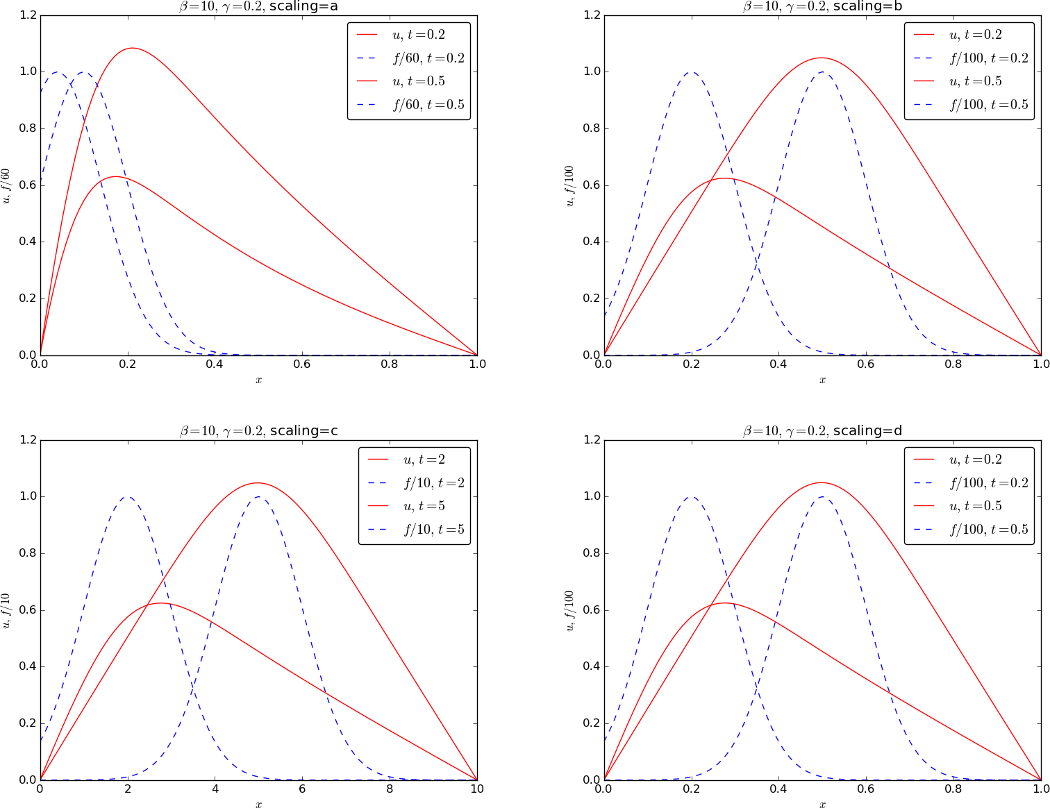
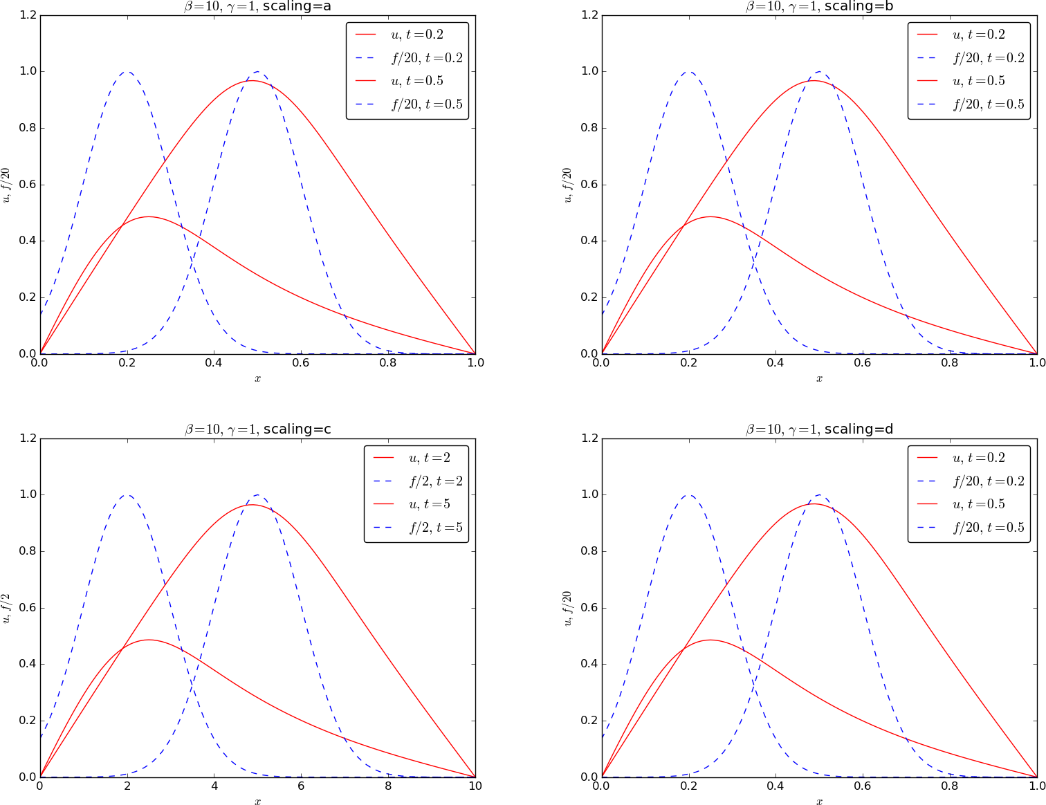
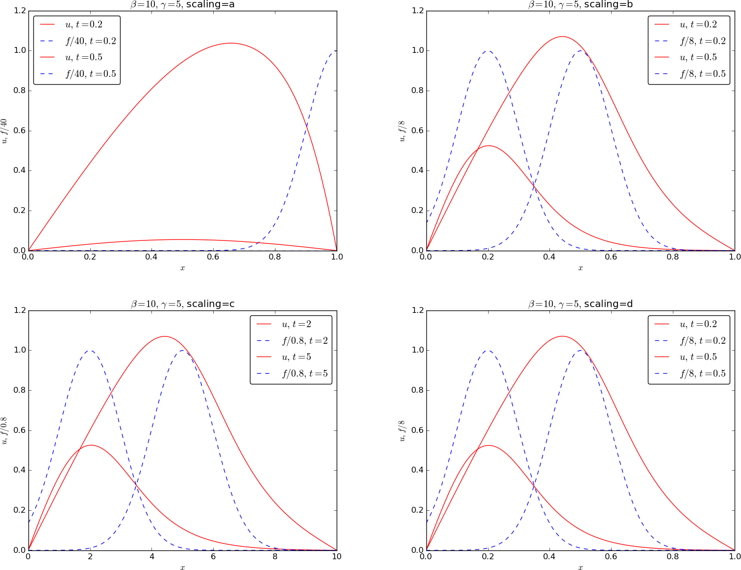
f) Use the software in e) to investigate \( \gamma=0.2,1,5,40 \) for the four scalings. Discuss the results.
For these investigations, we compare the three scalings for each of the different \( \gamma \) values. An appropriate function for automating the tasks is
def investigate():
    """Do scienfic experiments with the run function above."""
    # Clean up old files
    import glob, os
    for filename in glob.glob('tmp1_gamma*') + \
            glob.glob('welding_gamma*'):
        os.remove(filename)

    scaling_values = 'abcd'
    gamma_values = 1, 40, 5, 0.2, 0.025
    delta_values = {}  # delta_values[scaling][gamma]
    delta_values['a'] = {0.025: 140, 0.2: 60,  1: 20, 5: 40,  40: 800}
    delta_values['b'] = {0.025: 700, 0.2: 100, 1: 20, 5: 8,   40: 5}
    delta_values['c'] = {0.025: 80,  0.2: 10,  1: 2,  5: 0.8, 40: 0.5}
    delta_values['d'] = {0.025: 20,  0.2: 20,  1: 20, 5: 40,  40: 200}
    for gamma in gamma_values:
        for scaling in scaling_values:
            run(gamma=gamma, beta=10,
                delta=delta_values[scaling][gamma],
                scaling=scaling)

    # Combine images
    for gamma in gamma_values:
        for ext in 'pdf', 'png':
            cmd = 'doconce combine_images -2'
            for s in scaling_values:
                cmd += ' tmp1_gamma%(gamma)g_%(s)s.%(ext)s ' % vars()
            cmd += ' welding_gamma%(gamma)g.%(ext)s' % vars()
            os.system(cmd)
            # pdflatex doesn't like a dot (as in 0.2) in filenames...
            if '.' in str(gamma):
                os.rename(
                'welding_gamma%(gamma)g.%(ext)s' % vars(),
                ('welding_gamma%(gamma)g' % vars()).replace('.', '_')
                + '.' + ext)
Note that for each \( \gamma \) value and each scaling, we have found
a \( \delta \) value such that the maximum \( u \) value is around unity in size.
We did this first by trial and error, and thereafter filled out the
delta_values dictionary.
The scalings in b)-d) are illustrated at the same physical times. The scaling in a) is plotted at the same non-dimensional time as used in the other scalings, but observe that this is a different physical time than used for the b)-d) scalings.
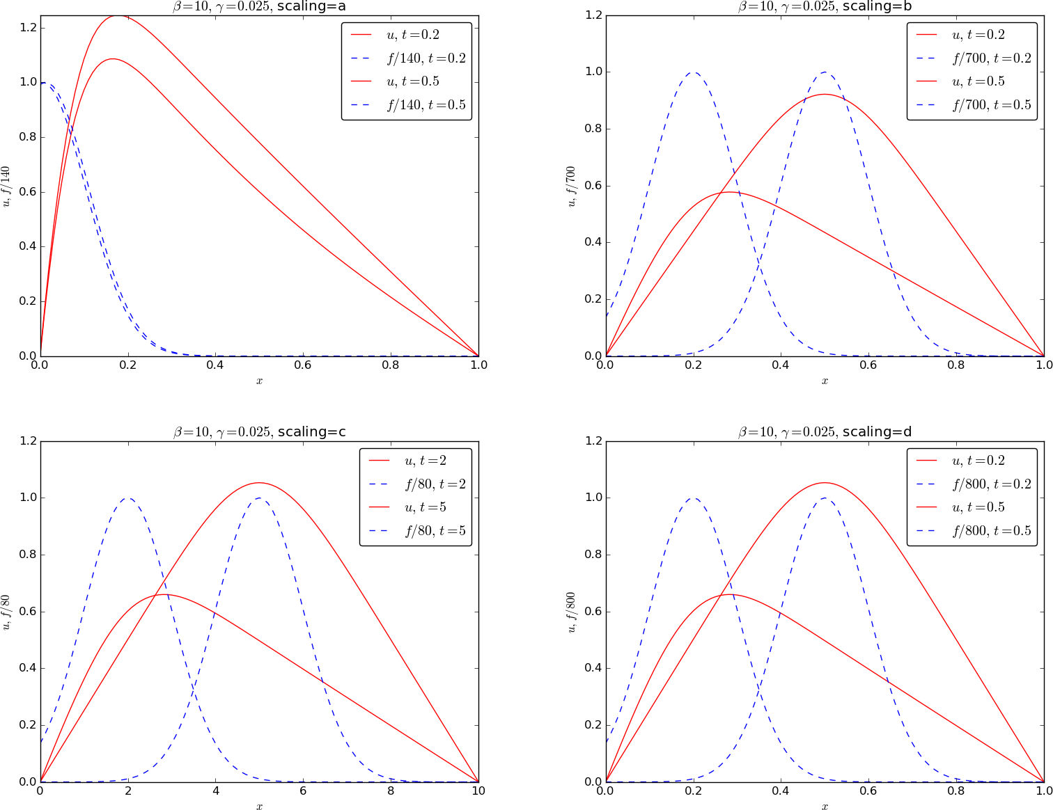
We get the following plots, with the a) and c) scalings to the left and the b) and d) scalings to the right, starting with \( \gamma=0.025 \) and increasing its value to \( \gamma=40 \):
\( \gamma=0.025 \). For small \( \gamma \), 0.025 and 0.2, the scales b)-d) are equally applicable, while the diffusion time scale, which is much longer, does not fit with the heat source motion.
Below are the results for \( \gamma=0.02 \).
For \( \gamma=1 \), all the scalings are equal and provide identical results.
Next we present results for \( \gamma=5 \).
Finally, we have the results for \( \gamma=40 \).

Discussion. From these plots we see that it does not matter which of the scalings in b)-d) we choose, as long as we compensate with the \( \delta \) parameter to bring \( u \) to the size of unity. The scaling a) is suitable for \( \gamma\leq 1 \), it seems, but graphs at earlier times for \( \gamma=5,40 \) should be investigated before drawing a conclusion.
Looking at the necessary values of \( \delta \) to bring \( u \) around the size of unity, and noting that the factor used to scale \( f \) is \( \delta/\gamma \) in scaling d), we see that for small \( \gamma \), the scaling in d) requires an adjustment \( \delta =20 \), while the scaling in b) requires \( \delta =700 \). For the large \( \gamma=40 \), the situation is opposite: the scaling in d) requires \( \delta=200 \), while the one in b) only needs \( \delta =5 \). The scaling in c) is very similar to the scaling in b), apart from the factor \( L/\sigma \) (times, \( \delta \), etc. are all differ by the factor \( L/\sigma \)).
We therefore conclude that the scaling in d) is best for small \( \gamma \) and the scaling b) is best for large \( \gamma \), but with the \( \delta \) trick used here, it really does not matter for practical calculations which scaling we use. Nevertheless, the insight given by the scalings should not be forgotten: we see in d) that for large \( \gamma \) the time-derivative term can be neglected and in b) that the conduction term can be neglected.
We must also remark that the boundary conditions reduce the physical relevance of the results as we force the scaled temperature down to zero at the end points. The temperature at the end points are much more "free", in reality, resulting in flatter curves than what we achieved above. This flattening would also demonstrate that the heat from the welding equipment is more efficiently conducted away toward the boundaries. However, for investigating the differences between different scalings, the choice of boundary conditions is not a key issue.
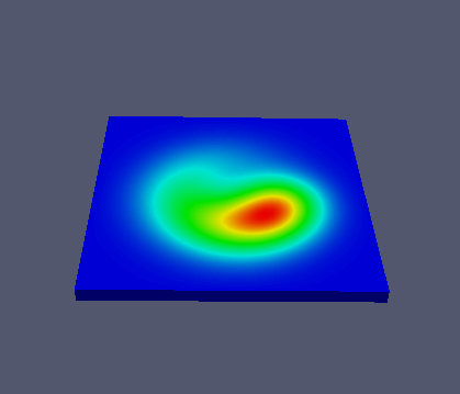
Simulations with a full 3D model. How relevant is it to study scaling in 1D model when we know that the heat loss from the material is not well modeled? We have implemented a full 3D model in the FEniCS programming system and performed simulations using cooling law boundary conditions (i.e., conditions of Robin type). In the dimensionless cooling law, we set the Nusselt number to 1. The other dimensionless parameters are as in the 1D problem, but the welding equipment moves in a circle rather along a line as it had to in the 1D problem.
Below is a plot of the heat source (upper left) and temperature distributions for \( \gamma=0.1 \) (upper right), \( \gamma=1 \) (lower left), and \( \gamma=30 \) (lower right), after two rotations.
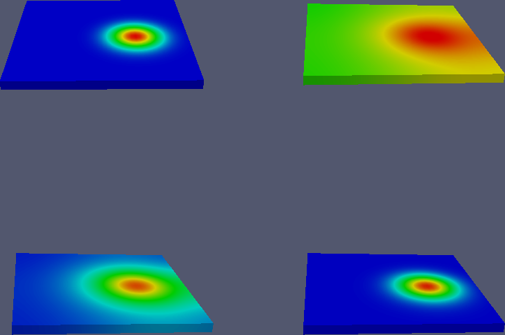
Gearing \( \gamma \) up to 2000 gives the following comet-like temperature distribution:
From the movies below we can clearly see how the temperature is effectively spreading in 3D for small \( \gamma \) values, while for large values the temperature hardly reaches the boundary.
\( \gamma=0.1 \).
\( \gamma=1 \).
\( \gamma=30 \).
\( \gamma=2000 \).
Filename: welding.