Vibration ODEs
Vibration problems lead to differential equations with solutions that oscillate in time, typically in a damped or undamped sinusoidal fashion. Such solutions put certain demands on the numerical methods compared to other phenomena whose solutions are monotone or very smooth. Both the frequency and amplitude of the oscillations need to be accurately handled by the numerical schemes. The forthcoming text presents a range of different methods, from classical ones (Runge-Kutta and midpoint/Crank-Nicolson methods), to more modern and popular symplectic (geometric) integration schemes (Leapfrog, Euler-Cromer, and Stoermer-Verlet methods), but with a clear emphasis on the latter. Vibration problems occur throughout mechanics and physics, but the methods discussed in this text are also fundamental for constructing successful algorithms for partial differential equations of wave nature in multiple spatial dimensions.
Finite difference discretization
Many of the numerical challenges faced when computing oscillatory solutions to ODEs and PDEs can be captured by the very simple ODE \(u^{\prime\prime} + u =0\). This ODE is thus chosen as our starting point for method development, implementation, and analysis.
A basic model for vibrations
The simplest model of a vibrating mechanical system has the following form:
Here, \(\omega\) and \(I\) are given constants. The section Oscillating mass attached to a spring derives (1) from physical principles and explains what the constants mean.
The exact solution of (1) is
That is, \(u\) oscillates with constant amplitude \(I\) and angular frequency \(\omega\). The corresponding period of oscillations (i.e., the time between two neighboring peaks in the cosine function) is \(P=2\pi/\omega\). The number of periods per second is \(f=\omega/(2\pi)\) and measured in the unit Hz. Both \(f\) and \(\omega\) are referred to as frequency, but \(\omega\) is more precisely named angular frequency, measured in rad/s.
In vibrating mechanical systems modeled by (1), \(u(t)\) very often represents a position or a displacement of a particular point in the system. The derivative \(u^{\prime}(t)\) then has the interpretation of velocity, and \(u^{\prime\prime}(t)\) is the associated acceleration. The model (1) is not only applicable to vibrating mechanical systems, but also to oscillations in electrical circuits.
A centered finite difference scheme
To formulate a finite difference method for the model problem (1) we follow the four steps explained in [Ref02].
Step 1: Discretizing the domain
The domain is discretized by introducing a uniformly partitioned time mesh. The points in the mesh are \(t_n=n\Delta t\), \(n=0,1,\ldots,N_t\), where \(\Delta t = T/N_t\) is the constant length of the time steps. We introduce a mesh function \(u^n\) for \(n=0,1,\ldots,N_t\), which approximates the exact solution at the mesh points. (Note that \(n=0\) is the known initial condition, so \(u^n\) is identical to the mathematical \(u\) at this point.) The mesh function \(u^n\) will be computed from algebraic equations derived from the differential equation problem.
Step 2: Fulfilling the equation at discrete time points
The ODE is to be satisfied at each mesh point where the solution must be found:
Step 3: Replacing derivatives by finite differences
The derivative \(u^{\prime\prime}(t_n)\) is to be replaced by a finite difference approximation. A common second-order accurate approximation to the second-order derivative is
We also need to replace the derivative in the initial condition by a finite difference. Here we choose a centered difference, whose accuracy is similar to the centered difference we used for \(u^{\prime\prime}\):
Step 4: Formulating a recursive algorithm
To formulate the computational algorithm, we assume that we have already computed \(u^{n-1}\) and \(u^n\), such that \(u^{n+1}\) is the unknown value to be solved for:
The computational algorithm is simply to apply (7) successively for \(n=1,2,\ldots,N_t-1\). This numerical scheme sometimes goes under the name Stoermer’s method, Verlet integration, or the Leapfrog method (one should note that Leapfrog is used for many quite different methods for quite different differential equations!).
Computing the first step
We observe that (7) cannot be used for \(n=0\) since the computation of \(u^1\) then involves the undefined value \(u^{-1}\) at \(t=-\Delta t\). The discretization of the initial condition then comes to our rescue: (6) implies \(u^{-1} = u^1\) and this relation can be combined with (7) for \(n=0\) to yield a value for \(u^1\):
which reduces to
Exercise 1.5: Use a Taylor polynomial to compute asks you to perform an alternative derivation and also to generalize the initial condition to \(u^{\prime}(0)=V\neq 0\).
The computational algorithm
The steps for solving (1) become
The algorithm is more precisely expressed directly in Python:
t = linspace(0, T, Nt+1)  # mesh points in time
dt = t[1] - t[0]          # constant time step
u = zeros(Nt+1)           # solution

u[0] = I
u[1] = u[0] - 0.5*dt**2*w**2*u[0]
for n in range(1, Nt):
    u[n+1] = 2*u[n] - u[n-1] - dt**2*w**2*u[n]
Remark on using w for \(\omega\) in computer code
In the code, we use w as the symbol for \(\omega\).
The reason is that the authors prefer w for readability
and comparison with the mathematical \(\omega\) instead of
the full word omega as variable name.
Operator notation
We may write the scheme using a compact difference notation listed in Finite difference operator notation (see also examples in [Ref02]). The difference (4) has the operator notation \([D_tD_t u]^n\) such that we can write:
Note that \([D_tD_t u]^n\) means applying a central difference with step \(\Delta t/2\) twice:
which is written out as
The discretization of initial conditions can in the operator notation be expressed as
where the operator \([D_{2t} u]^n\) is defined as
Implementation
Making a solver function
The algorithm from the previous section is readily translated to a complete Python function for computing and returning \(u^0,u^1,\ldots,u^{N_t}\) and \(t_0,t_1,\ldots,t_{N_t}\), given the input \(I\), \(\omega\), \(\Delta t\), and \(T\):
import numpy as np
import matplotlib.pyplot as plt

def solver(I, w, dt, T):
    """
    Solve u'' + w**2*u = 0 for t in (0,T], u(0)=I and u'(0)=0,
    by a central finite difference method with time step dt.
    """
    dt = float(dt)
    Nt = int(round(T/dt))
    u = np.zeros(Nt+1)
    t = np.linspace(0, Nt*dt, Nt+1)

    u[0] = I
    u[1] = u[0] - 0.5*dt**2*w**2*u[0]
    for n in range(1, Nt):
        u[n+1] = 2*u[n] - u[n-1] - dt**2*w**2*u[n]
    return u, t
We have imported numpy and matplotlib under the names np and plt,
respectively, as this is very common in the Python scientific
computing community and a good programming habit (since we explicitly
see where the different functions come from). An alternative is to do
from numpy import * and a similar “import all” for Matplotlib to
avoid the np and plt prefixes and make the code as close as
possible to MATLAB. (See the section
Prefixing imported functions by the module name in the book
Finite Difference Computing with Exponential Decay Models [Ref02] for a discussion of the two
types of import in Python.)
A function for plotting the numerical and the exact solution is also convenient to have:
def u_exact(t, I, w):
    return I*np.cos(w*t)

def visualize(u, t, I, w):
    plt.plot(t, u, 'r--o')
    t_fine = np.linspace(0, t[-1], 1001)  # very fine mesh for u_e
    u_e = u_exact(t_fine, I, w)
    plt.hold('on')
    plt.plot(t_fine, u_e, 'b-')
    plt.legend(['numerical', 'exact'], loc='upper left')
    plt.xlabel('t')
    plt.ylabel('u')
    dt = t[1] - t[0]
    plt.title('dt=%g' % dt)
    umin = 1.2*u.min();  umax = -umin
    plt.axis([t[0], t[-1], umin, umax])
    plt.savefig('tmp1.png');  plt.savefig('tmp1.pdf')
A corresponding main program calling these functions to simulate
a given number of periods (num_periods) may take the form
I = 1
w = 2*pi
dt = 0.05
num_periods = 5
P = 2*pi/w    #  one period
T = P*num_periods
u, t = solver(I, w, dt, T)
visualize(u, t, I, w, dt)
Adjusting some of the input parameters via the command line can be
handy. Here is a code segment using the ArgumentParser tool in
the argparse module to define option value (--option value)
pairs on the command line:
import argparse
parser = argparse.ArgumentParser()
parser.add_argument('--I', type=float, default=1.0)
parser.add_argument('--w', type=float, default=2*pi)
parser.add_argument('--dt', type=float, default=0.05)
parser.add_argument('--num_periods', type=int, default=5)
a = parser.parse_args()
I, w, dt, num_periods = a.I, a.w, a.dt, a.num_periods
- Such parsing of the command line is explained in more detail in
- the
section Option-value pairs on the command line in Finite Difference Computing with Exponential Decay Models [Ref02].
A typical execution goes like
Terminal> python vib_undamped.py --num_periods 20 --dt 0.1
Computing \(u^{\prime}\)
In mechanical vibration applications one is often interested in computing the velocity \(v(t)=u^{\prime}(t)\) after \(u(t)\) has been computed. This can be done by a central difference,
This formula applies for all inner mesh points, \(n=1,\ldots,N_t-1\). For \(n=0\), \(v(0)\) is given by the initial condition on \(u^{\prime}(0)\), and for \(n=N_t\) we can use a one-sided, backward difference:
Typical (scalar) code is
v = np.zeros_like(u)  # or v = np.zeros(len(u))
# Use central difference for internal points
for i in range(1, len(u)-1):
    v[i] = (u[i+1] - u[i-1])/(2*dt)
# Use initial condition for u'(0) when i=0
v[0] = 0
# Use backward difference at the final mesh point
v[-1] = (u[-1] - u[-2])/dt
Since the loop is slow for large \(N_t\), we can get rid of the loop by vectorizing the central difference. The above code segment goes as follows in its vectorized version (see the problem Differentiate a function in Finite Difference Computing with Exponential Decay Models [Ref02] for explanation of details):
v = np.zeros_like(u)
v[1:-1] = (u[2:] - u[:-2])/(2*dt)  # central difference
v[0] = 0                           # boundary condition u'(0)
v[-1] = (u[-1] - u[-2])/dt         # backward difference
Verification
Manual calculation
The simplest type of verification, which is also instructive for understanding
the algorithm, is to compute \(u^1\), \(u^2\), and \(u^3\)
with the aid of a calculator
and make a function for comparing these results with those from the solver
function. The test_three_steps function in
the file vib_undamped.py
shows the details of how we use the hand calculations to test the code:
def test_three_steps():
    from math import pi
    I = 1;  w = 2*pi;  dt = 0.1;  T = 1
    u_by_hand = np.array([1.000000000000000,
                          0.802607911978213,
                          0.288358920740053])
    u, t = solver(I, w, dt, T)
    diff = np.abs(u_by_hand - u[:3]).max()
    tol = 1E-14
    assert diff < tol
This function is a proper test function, compliant with the pytest and nose testing framework for Python code, because
- the function name begins with
test_- the function takes no arguments
- the test is formulated as a boolean condition and executed by
assert
We shall in this book implement all software verification via such
proper test functions, also known as unit testing.
See the
section Unit tests and test functions in
Finite Difference Computing with Exponential Decay Models [Ref02]
for more details on how to construct test functions and utilize nose
or pytest for automatic execution of tests. Our recommendation is to
use pytest. With this choice, you can
run all test functions in vib_undamped.py by
Terminal> py.test -s -v vib_undamped.py
============================= test session starts ======...
platform linux2 -- Python 2.7.9 -- ...
collected 2 items

vib_undamped.py::test_three_steps PASSED
vib_undamped.py::test_convergence_rates PASSED

=========================== 2 passed in 0.19 seconds ===...
Testing very simple polynomial solutions
Constructing test problems where the exact solution is constant or linear helps initial debugging and verification as one expects any reasonable numerical method to reproduce such solutions to machine precision. Second-order accurate methods will often also reproduce a quadratic solution. Here \([D_tD_tt^2]^n=2\), which is the exact result. A solution \(u=t^2\) leads to \(u^{\prime\prime}+\omega^2 u=2 + (\omega t)^2\neq 0\). We must therefore add a source in the equation: \(u^{\prime\prime} + \omega^2 u = f\) to allow a solution \(u=t^2\) for \(f=2 + (\omega t)^2\). By simple insertion we can show that the mesh function \(u^n = t_n^2\) is also a solution of the discrete equations. Problem 1.1: Use linear/quadratic functions for verification asks you to carry out all details to show that linear and quadratic solutions are solutions of the discrete equations. Such results are very useful for debugging and verification. You are strongly encouraged to do this problem now!
Checking convergence rates
Empirical computation of convergence rates yields a good method for verification. The method and its computational details are explained in detail for a simple ODE model in the section Computing convergence rates in Finite Difference Computing with Exponential Decay Models [Ref02]. Readers not familiar with the concept should look up this reference before proceeding.
In the present problem, computing convergence rates means that we must
- perform \(m\) simulations, halving the time steps as: \(\Delta t_i=2^{-i}\Delta t_0\), \(i=1,\ldots,m-1\), and \(\Delta t_i\) is the time step used in simulation \(i\);
- compute the \(L^2\) norm of the error, \(E_i=\sqrt{\Delta t_i\sum_{n=0}^{N_t-1}(u^n-{u_{\small\mbox{e}}}(t_n))^2}\) in each case;
- estimate the convergence rates \(r_i\) based on two consecutive experiments \((\Delta t_{i-1}, E_{i-1})\) and \((\Delta t_{i}, E_{i})\), assuming \(E_i=C(\Delta t_i)^{r}\) and \(E_{i-1}=C(\Delta t_{i-1})^{r}\). From these equations it follows that \(r = \ln (E_{i-1}/E_i)/\ln (\Delta t_{i-1}/\Delta t_i)\). Since this \(r\) will vary with \(i\), we equip it with an index and call it \(r_{i-1}\), where \(i\) runs from \(1\) to \(m-1\).
The computed rates \(r_0,r_1,\ldots,r_{m-2}\) hopefully converge to the number 2 in the present problem, because theory (from the section Analysis of the numerical scheme) shows that the error of the numerical method we use behaves like \(\Delta t^2\). The convergence of the sequence \(r_0,r_1,\ldots,r_{m-2}\) demands that the time steps \(\Delta t_i\) are sufficiently small for the error model \(E_i=C(\Delta t_i)^r\) to be valid.
All the implementational details of computing the sequence \(r_0,r_1,\ldots,r_{m-2}\) appear below.
def convergence_rates(m, solver_function, num_periods=8):
    """
    Return m-1 empirical estimates of the convergence rate
    based on m simulations, where the time step is halved
    for each simulation.
    solver_function(I, w, dt, T) solves each problem, where T
    is based on simulation for num_periods periods.
    """
    from math import pi
    w = 0.35; I = 0.3       # just chosen values
    P = 2*pi/w              # period
    dt = P/30               # 30 time step per period 2*pi/w
    T = P*num_periods

    dt_values = []
    E_values = []
    for i in range(m):
        u, t = solver_function(I, w, dt, T)
        u_e = u_exact(t, I, w)
        E = np.sqrt(dt*np.sum((u_e-u)**2))
        dt_values.append(dt)
        E_values.append(E)
        dt = dt/2

    r = [np.log(E_values[i-1]/E_values[i])/
         np.log(dt_values[i-1]/dt_values[i])
         for i in range(1, m, 1)]
    return r, E_values, dt_values
The error analysis in the section Analysis of the numerical scheme is quite detailed and suggests that \(r=2\). It is also a intuitively reasonable result, since we used a second-order accurate finite difference approximation \([D_tD_tu]^n\) to the ODE and a second-order accurate finite difference formula for the initial condition for \(u^{\prime}\).
In the present problem, when \(\Delta t_0\) corresponds to 30 time steps
per period, the returned r list has all its values equal to 2.00
(if rounded to two decimals). This amazingly accurate result means that all
\(\Delta t_i\) values are well into the asymptotic regime where the
error model \(E_i = C(\Delta t_i)^r\) is valid.
We can now construct a proper test function that computes convergence rates and checks that the final (and usually the best) estimate is sufficiently close to 2. Here, a rough tolerance of 0.1 is enough. This unit test goes like
def test_convergence_rates():
    r, E, dt = convergence_rates(
        m=5, solver_function=solver, num_periods=8)
    # Accept rate to 1 decimal place
    tol = 0.1
    assert abs(r[-1] - 2.0) < tol
    # Test that adjusted w obtains 4th order convergence
    r, E, dt = convergence_rates(
        m=5, solver_function=solver_adjust_w, num_periods=8)
    print 'adjust w rates:', r
    assert abs(r[-1] - 4.0) < tol
The complete code appears in the file vib_undamped.py.
Visualizing convergence rates with slope markers
Tony S. Yu has written a script plotslopes.py
that is very useful to indicate the slope of a graph, especially
a graph like \(\ln E = r\ln \Delta t + \ln C\) arising from the model
\(E=C\Delta t^r\). A copy of the script resides in the src/vib
directory. Let us use it to compare the original method for \(u'' + \omega^2u =0\)
with the same method applied to the equation with a modified
\(\omega\). We make log-log plots of the error versus \(\Delta t\).
For each curve we attach a slope marker using the slope_marker((x,y), r)
function from plotslopes.py, where (x,y) is the position of the
marker and r and the slope (\((r,1)\)), here (2,1) and (4,1).
def plot_convergence_rates():
    r2, E2, dt2 = convergence_rates(
        m=5, solver_function=solver, num_periods=8)
    plt.loglog(dt2, E2)
    r4, E4, dt4 = convergence_rates(
        m=5, solver_function=solver_adjust_w, num_periods=8)
    plt.loglog(dt4, E4)
    plt.legend(['original scheme', r'adjusted $\omega$'],
               loc='upper left')
    plt.title('Convergence of finite difference methods')
    from plotslopes import slope_marker
    slope_marker((dt2[1], E2[1]), (2,1))
    slope_marker((dt4[1], E4[1]), (4,1))
Figure Empirical convergence rate curves with special slope marker displays the two curves with the markers. The match of the curve slope and the marker slope is excellent.
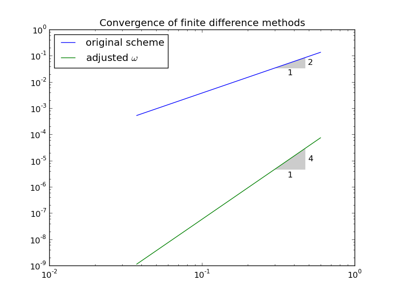
Empirical convergence rate curves with special slope marker
Scaled model
It is advantageous to use dimensionless variables in simulations, because fewer parameters need to be set. The present problem is made dimensionless by introducing dimensionless variables \(\bar t = t/t_c\) and \(\bar u = u/u_c\), where \(t_c\) and \(u_c\) are characteristic scales for \(t\) and \(u\), respectively. We refer to the section Undamped vibrations without forcing in the book Scaling of differential equations [Ref03] for all details about this scaling.
The scaled ODE problem reads
A common choice is to take \(t_c\) as one period of the oscillations, \(t_c = 2\pi/w\), and \(u_c=I\). This gives the dimensionless model
Observe that there are no physical parameters in (13)! We can therefore perform a single numerical simulation \(\bar u(\bar t)\) and afterwards recover any \(u(t; \omega, I)\) by
We can easily check this assertion: the solution of the scaled problem is \(\bar u(\bar t) = \cos(2\pi\bar t)\). The formula for \(u\) in terms of \(\bar u\) gives \(u = I\cos(\omega t)\), which is nothing but the solution of the original problem with dimensions.
The scaled model can by run by calling solver(I=1, w=2*pi, dt, T).
Each period is now 1 and T simply counts the number of periods.
Choosing dt as 1./M gives M time steps per period.
Visualization of long time simulations
Figure Effect of halving the time step shows a comparison of the exact and numerical solution for the scaled model (13) with \(\Delta t=0.1, 0.05\). From the plot we make the following observations:
- The numerical solution seems to have correct amplitude.
- There is an angular frequency error which is reduced by decreasing the time step.
- The total angular frequency error grows with time.
By angular frequency error we mean that the numerical angular frequency differs from the exact \(\omega\). This is evident by looking at the peaks of the numerical solution: these have incorrect positions compared with the peaks of the exact cosine solution. The effect can be mathematically expressed by writing the numerical solution as \(I\cos\tilde\omega t\), where \(\tilde\omega\) is not exactly equal to \(\omega\). Later, we shall mathematically quantify this numerical angular frequency \(\tilde\omega\).
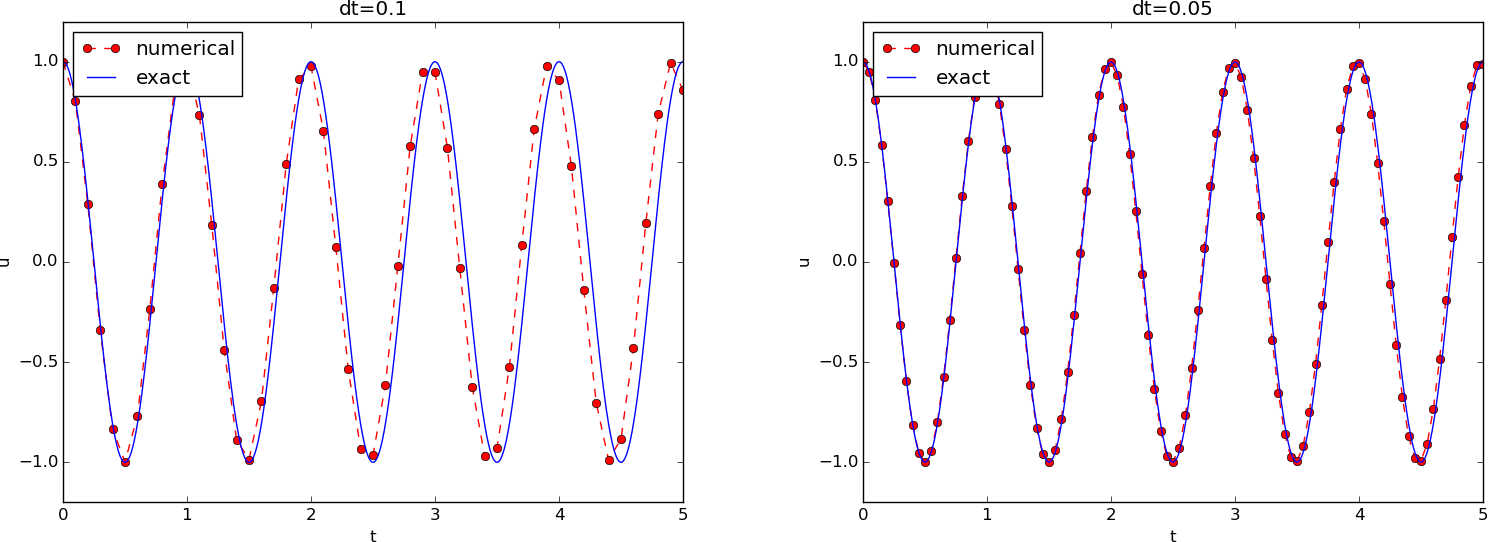
Effect of halving the time step
Using a moving plot window
In vibration problems it is often of interest to investigate the system’s
behavior over long time intervals. Errors in the angular frequency accumulate
and become more visible as time grows. We can investigate long
time series by introducing a moving plot window that can move along with
the \(p\) most recently computed periods of the solution. The
SciTools package contains
a convenient tool for this: MovingPlotWindow. Typing
pydoc scitools.MovingPlotWindow shows a demo and a description of its use.
The function below utilizes the moving plot window and is in fact
called by the main function in the vib_undamped module
if the number of periods in the simulation exceeds 10.
def visualize_front(u, t, I, w, savefig=False, skip_frames=1):
    """
    Visualize u and the exact solution vs t, using a
    moving plot window and continuous drawing of the
    curves as they evolve in time.
    Makes it easy to plot very long time series.
    Plots are saved to files if savefig is True.
    Only each skip_frames-th plot is saved (e.g., if
    skip_frame=10, only each 10th plot is saved to file;
    this is convenient if plot files corresponding to
    different time steps are to be compared).
    """
    import scitools.std as st
    from scitools.MovingPlotWindow import MovingPlotWindow
    from math import pi

    # Remove all old plot files tmp_*.png
    import glob, os
    for filename in glob.glob('tmp_*.png'):
        os.remove(filename)

    P = 2*pi/w  # one period
    umin = 1.2*u.min();  umax = -umin
    dt = t[1] - t[0]
    plot_manager = MovingPlotWindow(
        window_width=8*P,
        dt=dt,
        yaxis=[umin, umax],
        mode='continuous drawing')
    frame_counter = 0
    for n in range(1,len(u)):
        if plot_manager.plot(n):
            s = plot_manager.first_index_in_plot
            st.plot(t[s:n+1], u[s:n+1], 'r-1',
                    t[s:n+1], I*cos(w*t)[s:n+1], 'b-1',
                    title='t=%6.3f' % t[n],
                    axis=plot_manager.axis(),
                    show=not savefig) # drop window if savefig
            if savefig and n % skip_frames == 0:
                filename = 'tmp_%04d.png' % frame_counter
                st.savefig(filename)
                print 'making plot file', filename, 'at t=%g' % t[n]
                frame_counter += 1
        plot_manager.update(n)
We run the scaled problem (the default values for the command-line arguments
--I and --w correspond to the scaled problem) for 40 periods with 20
time steps per period:
Terminal> python vib_undamped.py --dt 0.05 --num_periods 40
The moving plot window is invoked, and we can follow the numerical and exact solutions as time progresses. From this demo we see that the angular frequency error is small in the beginning, and that it becomes more prominent with time. A new run with \(\Delta t=0.1\) (i.e., only 10 time steps per period) clearly shows that the phase errors become significant even earlier in the time series, deteriorating the solution further.
Making animations
Producing standard video formats
The visualize_front function stores all the plots in
files whose names are numbered:
tmp_0000.png, tmp_0001.png, tmp_0002.png,
and so on. From these files we may make a movie. The Flash
format is popular,
Terminal> ffmpeg -r 25 -i tmp_%04d.png -c:v flv movie.flv
The ffmpeg program can be replaced by the avconv program in
the above command if desired (but at the time of this writing it seems
to be more momentum in the ffmpeg project).
The -r option should come first and
describes the number of frames per second in the movie (even if we
would like to have slow movies, keep this number as large as 25,
otherwise files are skipped from the movie). The
-i option describes the name of the plot files.
Other formats can be generated by changing the video codec
and equipping the video file with the right extension:
| Format | Codec and filename |
|---|---|
| Flash | -c:v flv movie.flv |
| MP4 | -c:v libx264 movie.mp4 |
| WebM | -c:v libvpx movie.webm |
| Ogg | -c:v libtheora movie.ogg |
The video file can be played by some video player like vlc, mplayer,
gxine, or totem, e.g.,
Terminal> vlc movie.webm
A web page can also be used to play the movie. Today’s standard is
to use the HTML5 video tag:
<video autoplay loop controls
       width='640' height='365' preload='none'>
<source src='movie.webm'  type='video/webm; codecs="vp8, vorbis"'>
</video>
Modern browsers do not support all of the video formats. MP4 is needed to successfully play the videos on Apple devices that use the Safari browser. WebM is the preferred format for Chrome, Opera, Firefox, and Internet Explorer v9+. Flash was a popular format, but older browsers that required Flash can play MP4. All browsers that work with Ogg can also work with WebM. This means that to have a video work in all browsers, the video should be available in the MP4 and WebM formats. The proper HTML code reads
<video autoplay loop controls
       width='640' height='365' preload='none'>
<source src='movie.mp4'   type='video/mp4;
 codecs="avc1.42E01E, mp4a.40.2"'>
<source src='movie.webm'  type='video/webm;
 codecs="vp8, vorbis"'>
</video>
The MP4 format should appear first to ensure that Apple devices will load the video correctly.
Caution: number the plot files correctly
To ensure that the individual plot frames are shown in correct order,
it is important to number the files with zero-padded numbers
(0000, 0001, 0002, etc.). The printf format %04d specifies an
integer in a field of width 4, padded with zeros from the left.
A simple Unix wildcard file specification like tmp_*.png
will then list the frames in the right order. If the numbers in the
filenames were not zero-padded, the frame tmp_11.png would appear
before tmp_2.png in the movie.
Playing PNG files in a web browser
The scitools movie command can create a movie player for a set
of PNG files such that a web browser can be used to watch the movie.
This interface has the advantage that the speed of the movie can
easily be controlled, a feature that scientists often appreciate.
The command for creating an HTML with a player for a set of
PNG files tmp_*.png goes like
Terminal> scitools movie output_file=vib.html fps=4 tmp_*.png
The fps argument controls the speed of the movie (“frames per second”).
To watch the movie, load the video file vib.html into some browser, e.g.,
Terminal> google-chrome vib.html # invoke web page
Clicking on Start movie to see the result. Moving this movie to
some other place requires moving vib.html and all the PNG files
tmp_*.png:
Terminal> mkdir vib_dt0.1
Terminal> mv tmp_*.png vib_dt0.1
Terminal> mv vib.html vib_dt0.1/index.html
Making animated GIF files
The convert program from the ImageMagick software suite can be
used to produce animated GIF files from a set of PNG files:
Terminal> convert -delay 25 tmp_vib*.png tmp_vib.gif
The -delay option needs an argument of the delay between each frame,
measured in 1/100 s, so 4 frames/s here gives 25/100 s delay.
Note, however, that in this particular example
with \(\Delta t=0.05\) and 40 periods,
making an animated GIF file out of
the large number of PNG files is a very heavy process and not
considered feasible. Animated GIFs are best suited for animations with
not so many frames and where you want to see each frame and play them
slowly.
Using Bokeh to compare graphs
Instead of a moving plot frame, one can use tools that allow panning by the mouse. For example, we can show four periods of several signals in several plots and then scroll with the mouse through the rest of the simulation simultaneously in all the plot windows. The Bokeh plotting library offers such tools, but the plots must be displayed in a web browser. The documentation of Bokeh is excellent, so here we just show how the library can be used to compare a set of \(u\) curves corresponding to long time simulations. (By the way, the guidance to correct pronunciation of Bokeh in the documentation and on Wikipedia is not directly compatible with a YouTube video...).
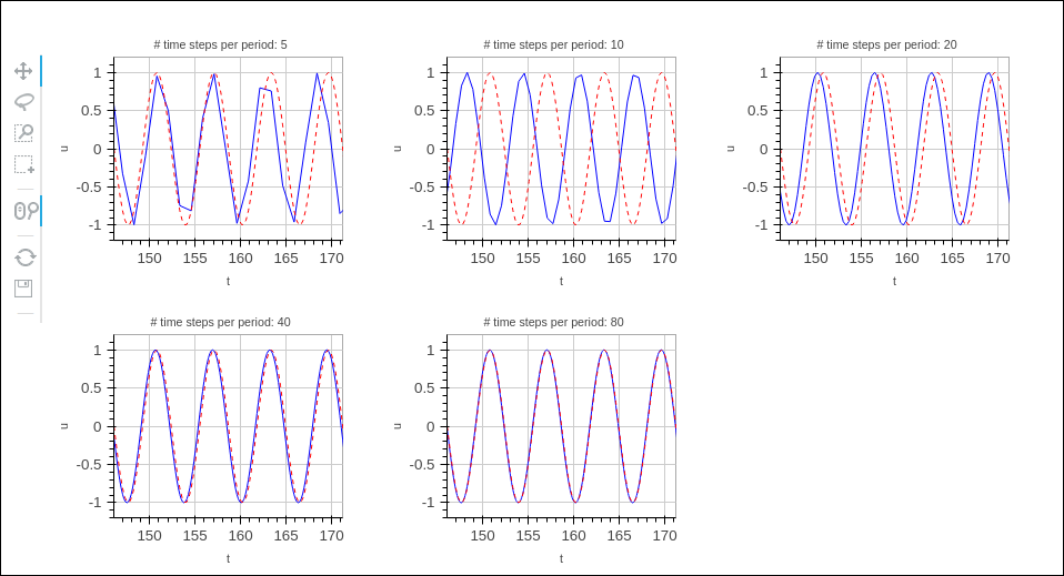
Imagine we have performed experiments for a set of \(\Delta t\) values. We want each curve, together with the exact solution, to appear in a plot, and then arrange all plots in a grid-like fashion:
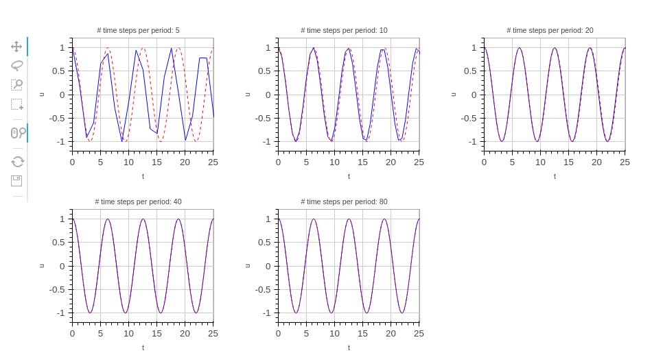
Furthermore, we want the axes to couple such that if we move into the future in one plot, all the other plots follows (note the displaced \(t\) axes!):
A function for creating a Bokeh plot, given a list of u arrays
and corresponding t arrays, is implemented below.
The code combines data fro different simulations, described
compactly in a list of strings legends.
def bokeh_plot(u, t, legends, I, w, t_range, filename):
    """
    Make plots for u vs t using the Bokeh library.
    u and t are lists (several experiments can be compared).
    legens contain legend strings for the various u,t pairs.
    """
    if not isinstance(u, (list,tuple)):
        u = [u]  # wrap in list
    if not isinstance(t, (list,tuple)):
        t = [t]  # wrap in list
    if not isinstance(legends, (list,tuple)):
        legends = [legends]  # wrap in list

    import bokeh.plotting as plt
    plt.output_file(filename, mode='cdn', title='Comparison')
    # Assume that all t arrays have the same range
    t_fine = np.linspace(0, t[0][-1], 1001)  # fine mesh for u_e
    tools = 'pan,wheel_zoom,box_zoom,reset,'\
            'save,box_select,lasso_select'
    u_range = [-1.2*I, 1.2*I]
    font_size = '8pt'
    p = []  # list of plot objects
    # Make the first figure
    p_ = plt.figure(
        width=300, plot_height=250, title=legends[0],
        x_axis_label='t', y_axis_label='u',
        x_range=t_range, y_range=u_range, tools=tools,
        title_text_font_size=font_size)
    p_.xaxis.axis_label_text_font_size=font_size
    p_.yaxis.axis_label_text_font_size=font_size
    p_.line(t[0], u[0], line_color='blue')
    # Add exact solution
    u_e = u_exact(t_fine, I, w)
    p_.line(t_fine, u_e, line_color='red', line_dash='4 4')
    p.append(p_)
    # Make the rest of the figures and attach their axes to
    # the first figure's axes
    for i in range(1, len(t)):
        p_ = plt.figure(
            width=300, plot_height=250, title=legends[i],
            x_axis_label='t', y_axis_label='u',
            x_range=p[0].x_range, y_range=p[0].y_range, tools=tools,
            title_text_font_size=font_size)
        p_.xaxis.axis_label_text_font_size = font_size
        p_.yaxis.axis_label_text_font_size = font_size
        p_.line(t[i], u[i], line_color='blue')
        p_.line(t_fine, u_e, line_color='red', line_dash='4 4')
        p.append(p_)

    # Arrange all plots in a grid with 3 plots per row
    grid = [[]]
    for i, p_ in enumerate(p):
        grid[-1].append(p_)
        if (i+1) % 3 == 0:
            # New row
            grid.append([])
    plot = plt.gridplot(grid, toolbar_location='left')
    plt.save(plot)
    plt.show(plot)
A particular example using the bokeh_plot function appears below.
def demo_bokeh():
    """Solve a scaled ODE u'' + u = 0."""
    from math import pi
    w = 1.0        # Scaled problem (frequency)
    P = 2*np.pi/w  # Period
    num_steps_per_period = [5, 10, 20, 40, 80]
    T = 40*P       # Simulation time: 40 periods
    u = []         # List of numerical solutions
    t = []         # List of corresponding meshes
    legends = []
    for n in num_steps_per_period:
        dt = P/n
        u_, t_ = solver(I=1, w=w, dt=dt, T=T)
        u.append(u_)
        t.append(t_)
        legends.append('# time steps per period: %d' % n)
    bokeh_plot(u, t, legends, I=1, w=w, t_range=[0, 4*P],
               filename='tmp.html')
Using a line-by-line ascii plotter
Plotting functions vertically, line by line, in the terminal window
using ascii characters only is a simple, fast, and convenient
visualization technique for long time series. Note that the time
axis then is positive downwards on the screen, so we can let the
solution be visualized “forever”.
The tool
scitools.avplotter.Plotter makes it easy to create such plots:
def visualize_front_ascii(u, t, I, w, fps=10):
    """
    Plot u and the exact solution vs t line by line in a
    terminal window (only using ascii characters).
    Makes it easy to plot very long time series.
    """
    from scitools.avplotter import Plotter
    import time
    from math import pi
    P = 2*pi/w
    umin = 1.2*u.min();  umax = -umin

    p = Plotter(ymin=umin, ymax=umax, width=60, symbols='+o')
    for n in range(len(u)):
        print p.plot(t[n], u[n], I*cos(w*t[n])), \
              '%.1f' % (t[n]/P)
        time.sleep(1/float(fps))
The call p.plot returns a line of text, with the \(t\) axis marked and
a symbol + for the first function (u) and o for the second
function (the exact solution). Here we append to this text
a time counter reflecting how many periods the current time point
corresponds to. A typical output (\(\omega =2\pi\), \(\Delta t=0.05\))
looks like this:
                         |                       o+      14.0
                         |                      + o      14.0
                         |                  +    o       14.1
                         |             +     o           14.1
                         |     +        o                14.2
                        +|       o                       14.2
                +        |                               14.2
         +       o       |                               14.3
    +     o              |                               14.4
 +   o                   |                               14.4
+o                       |                               14.5
o +                      |                               14.5
 o    +                  |                               14.6
     o      +            |                               14.6
          o        +     |                               14.7
                 o       | +                             14.7
                         |        +                      14.8
                         |       o       +               14.8
                         |              o     +          14.9
                         |                   o   +       14.9
                         |                       o+      15.0
Empirical analysis of the solution
For oscillating functions like those in Figure Effect of halving the time step we may compute the amplitude and frequency (or period) empirically. That is, we run through the discrete solution points \((t_n, u_n)\) and find all maxima and minima points. The distance between two consecutive maxima (or minima) points can be used as estimate of the local period, while half the difference between the \(u\) value at a maximum and a nearby minimum gives an estimate of the local amplitude.
The local maxima are the points where
and the local minima are recognized by
In computer code this becomes
def minmax(t, u):
    minima = []; maxima = []
    for n in range(1, len(u)-1, 1):
        if u[n-1] > u[n] < u[n+1]:
            minima.append((t[n], u[n]))
        if u[n-1] < u[n] > u[n+1]:
            maxima.append((t[n], u[n]))
    return minima, maxima
Note that the two returned objects are lists of tuples.
Let \((t_i, e_i)\), \(i=0,\ldots,M-1\), be the sequence of all the \(M\) maxima points, where \(t_i\) is the time value and \(e_i\) the corresponding \(u\) value. The local period can be defined as \(p_i=t_{i+1}-t_i\). With Python syntax this reads
def periods(maxima):
    p = [extrema[n][0] - maxima[n-1][0]
         for n in range(1, len(maxima))]
    return np.array(p)
The list p created by a list comprehension is converted to an array
since we probably want to compute with it, e.g., find the corresponding
frequencies 2*pi/p.
Having the minima and the maxima, the local amplitude can be calculated as the difference between two neighboring minimum and maximum points:
def amplitudes(minima, maxima):
    a = [(abs(maxima[n][1] - minima[n][1]))/2.0
         for n in range(min(len(minima),len(maxima)))]
    return np.array(a)
The code segments are found in the file vib_empirical_analysis.py.
Since a[i] and p[i] correspond to
the \(i\)-th amplitude estimate and the \(i\)-th period estimate, respectively,
it is most convenient to visualize the a and p values with the
index i on the horizontal axis.
(There is no unique time point associated with either of these estimate
since values at two different time points were used in the
computations.)
In the analysis of very long time series, it is advantageous to
compute and plot p and a instead of \(u\) to get an impression of
the development of the oscillations. Let us do this for the scaled
problem and \(\Delta t=0.1, 0.05, 0.01\).
A ready-made function
plot_empirical_freq_and_amplitude(u, t, I, w)
computes the empirical amplitudes and periods, and creates a plot
where the amplitudes and angular frequencies
are visualized together with the exact amplitude I
and the exact angular frequency w. We can make a little program
for creating the plot:
from vib_undamped import solver, plot_empirical_freq_and_amplitude
from math import pi
dt_values = [0.1, 0.05, 0.01]
u_cases = []
t_cases = []
for dt in dt_values:
    # Simulate scaled problem for 40 periods
    u, t = solver(I=1, w=2*pi, dt=dt, T=40)
    u_cases.append(u)
    t_cases.append(t)
plot_empirical_freq_and_amplitude(u_cases, t_cases, I=1, w=2*pi)
Figure Empirical angular frequency (left) and amplitude (right) for three different time steps shows the result: we clearly see that lowering \(\Delta t\) improves the angular frequency significantly, while the amplitude seems to be more accurate. The lines with \(\Delta t=0.01\), corresponding to 100 steps per period, can hardly be distinguished from the exact values. The next section shows how we can get mathematical insight into why amplitudes are good while frequencies are more inaccurate.
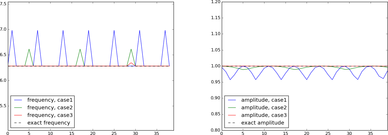
Empirical angular frequency (left) and amplitude (right) for three different time steps
Analysis of the numerical scheme
Deriving a solution of the numerical scheme
After having seen the phase error grow with time in the previous section, we shall now quantify this error through mathematical analysis. The key tool in the analysis will be to establish an exact solution of the discrete equations. The difference equation (7) has constant coefficients and is homogeneous. Such equations are known to have solutions on the form \(u^n=CA^n\), where \(A\) is some number to be determined from the difference equation and \(C\) is found as the initial condition (\(C=I\)). Recall that \(n\) in \(u^n\) is a superscript labeling the time level, while \(n\) in \(A^n\) is an exponent.
With oscillating functions as solutions, the algebra will be considerably simplified if we seek an \(A\) on the form
and solve for the numerical frequency \(\tilde\omega\) rather than \(A\). Note that \(i=\sqrt{-1}\) is the imaginary unit. (Using a complex exponential function gives simpler arithmetics than working with a sine or cosine function.) We have
The physically relevant numerical solution can be taken as the real part of this complex expression.
The calculations go as
The last line follows from the relation
\(\cos x - 1 = -2\sin^2(x/2)\) (try cos(x)-1 in
wolframalpha.com to see the formula).
The scheme (7) with \(u^n=Ie^{i\tilde\omega\Delta t\, n}\) inserted now gives
which after dividing by \(Ie^{i\tilde\omega t_n}\) results in
The first step in solving for the unknown \(\tilde\omega\) is
Then, taking the square root, applying the inverse sine function, and multiplying by \(2/\Delta t\), results in
The error in the numerical frequency
The first observation of (18) tells that there is a phase error since the numerical frequency \(\tilde\omega\) never equals the exact frequency \(\omega\). But how good is the approximation (18)? That is, what is the error \(\omega - \tilde\omega\) or \(\tilde\omega/\omega\)? Taylor series expansion for small \(\Delta t\) may give an expression that is easier to understand than the complicated function in (18):
>>> from sympy import *
>>> dt, w = symbols('dt w')
>>> w_tilde_e = 2/dt*asin(w*dt/2)
>>> w_tilde_series = w_tilde_e.series(dt, 0, 4)
>>> print w_tilde_series
w + dt**2*w**3/24 + O(dt**4)
This means that
The error in the numerical frequency is of second-order in \(\Delta t\), and the error vanishes as \(\Delta t\rightarrow 0\). We see that \(\tilde\omega > \omega\) since the term \(\omega^3\Delta t^2/24 >0\) and this is by far the biggest term in the series expansion for small \(\omega\Delta t\). A numerical frequency that is too large gives an oscillating curve that oscillates too fast and therefore “lags behind” the exact oscillations, a feature that can be seen in the left plot in Figure Effect of halving the time step.
Figure Exact discrete frequency and its second-order series expansion plots the discrete frequency (18) and its approximation (19) for \(\omega =1\) (based on the program vib_plot_freq.py). Although \(\tilde\omega\) is a function of \(\Delta t\) in (19), it is misleading to think of \(\Delta t\) as the important discretization parameter. It is the product \(\omega\Delta t\) that is the key discretization parameter. This quantity reflects the number of time steps per period of the oscillations. To see this, we set \(P=N_P\Delta t\), where \(P\) is the length of a period, and \(N_P\) is the number of time steps during a period. Since \(P\) and \(\omega\) are related by \(P=2\pi/\omega\), we get that \(\omega\Delta t = 2\pi/N_P\), which shows that \(\omega\Delta t\) is directly related to \(N_P\).
The plot shows that at least \(N_P\sim 25-30\) points per period are necessary for reasonable accuracy, but this depends on the length of the simulation (\(T\)) as the total phase error due to the frequency error grows linearly with time (see Exercise 1.2: Show linear growth of the phase with time).
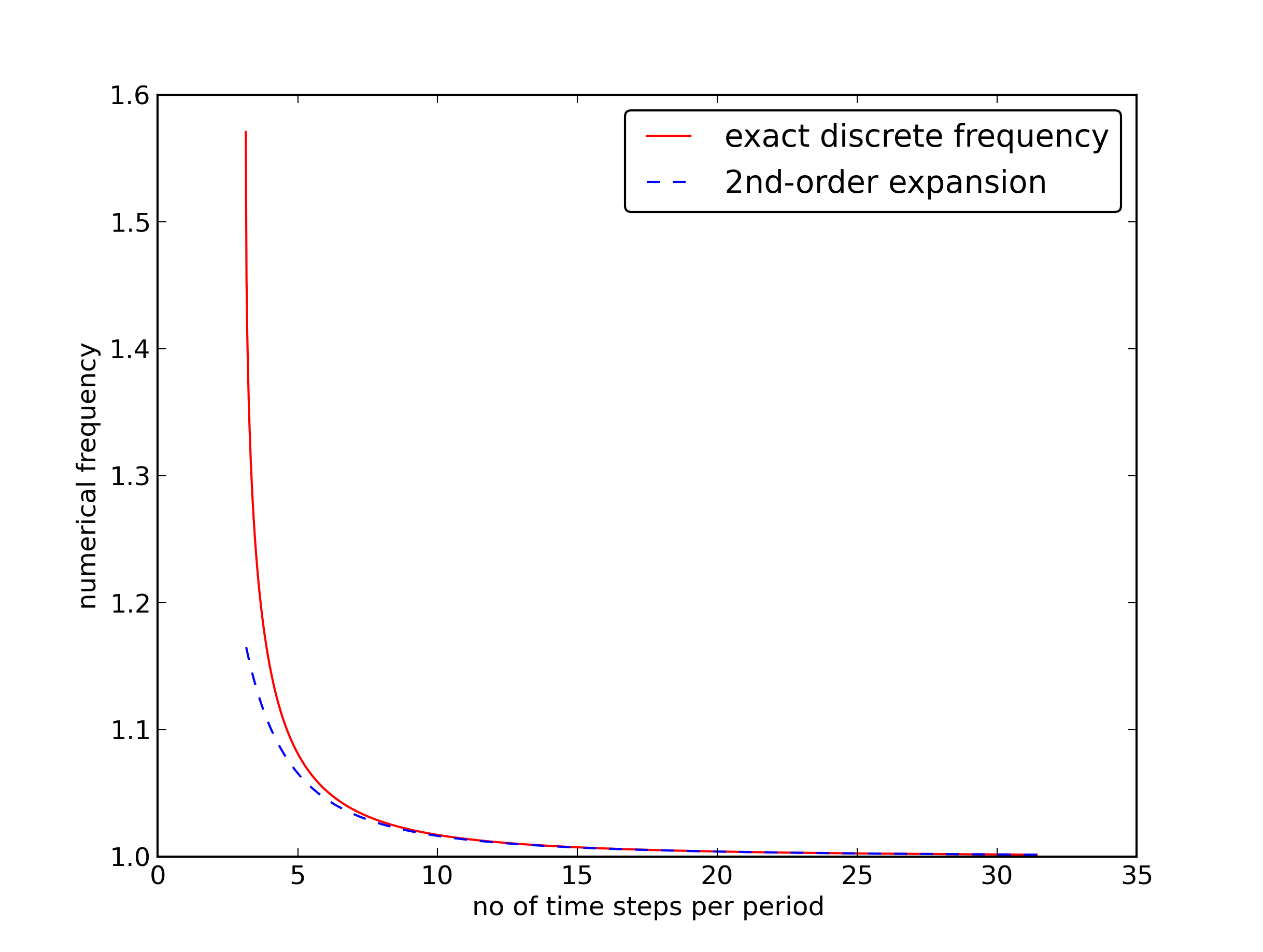
Exact discrete frequency and its second-order series expansion
Empirical convergence rates and adjusted \(\omega\)
The expression (19) suggest that adjusting omega to
could have effect on the convergence rate of the global error in \(u\)
(cf. the section Verification). With the convergence_rates function
in vib_undamped.py we can easily check this. A special solver, with
adjusted \(w\), is available as the function solver_adjust_w. A
call to convergence_rates with this solver reveals that the rate is
4.0! With the original, physical \(\omega\) the rate is 2.0 - as expected
from using second-order finite difference approximations,
as expected from the forthcoming derivation of the global error,
and as expected from truncation error analysis
analysis as explained in Linear model without damping.
Adjusting \(\omega\) is an ideal trick for this simple problem, but when adding damping and nonlinear terms, we have no simple formula for the impact on \(\omega\), and therefore we cannot use the trick.
Exact discrete solution
Perhaps more important than the \(\tilde\omega = \omega + {\cal O}(\Delta t^2)\) result found above is the fact that we have an exact discrete solution of the problem:
We can then compute the error mesh function
From the formula \(\cos 2x - \cos 2y = -2\sin(x-y)\sin(x+y)\) we can rewrite \(e^n\) so the expression is easier to interpret:
The error mesh function is ideal for verification purposes and you are strongly encouraged to make a test based on (20) by doing Exercise 1.11: Use an exact discrete solution for verification.
Convergence
We can use (19), (21), or (22) to show convergence of the numerical scheme, i.e., \(e^n\rightarrow 0\) as \(\Delta t\rightarrow 0\), which implies that the numerical solution approaches the exact solution as \(\Delta t\) approaches to zero. We have that
by L’Hopital’s rule. This result could also been computed WolframAlpha, or
we could use the limit functionality in sympy:
>>> import sympy as sym
>>> dt, w = sym.symbols('x w')
>>> sym.limit((2/dt)*sym.asin(w*dt/2), dt, 0, dir='+')
w
Also (19) can be used to establish that \(\tilde\omega\rightarrow\omega\) when \(\Delta t\rightarrow 0\). It then follows from the expression(s) for \(e^n\) that \(e^n\rightarrow 0\).
The global error
To achieve more analytical insight into the nature of the global
error, we can Taylor expand the error mesh function
(21). Since \(\tilde\omega\) in
(18) contains \(\Delta t\) in the denominator we
use the series expansion for \(\tilde\omega\) inside the cosine
function. A relevant sympy session is
>>> from sympy import *
>>> dt, w, t = symbols('dt w t')
>>> w_tilde_e = 2/dt*asin(w*dt/2)
>>> w_tilde_series = w_tilde_e.series(dt, 0, 4)
>>> w_tilde_series
w + dt**2*w**3/24 + O(dt**4)
Series expansions in sympy have the inconvenient O() term that
prevents further calculations with the series. We can use the
removeO() command to get rid of the O() term:
>>> w_tilde_series = w_tilde_series.removeO()
>>> w_tilde_series
dt**2*w**3/24 + w
Using this w_tilde_series expression for \(\tilde w\) in
(21), dropping \(I\) (which is a common factor), and
performing a series expansion of the error yields
>>> error = cos(w*t) - cos(w_tilde_series*t)
>>> error.series(dt, 0, 6)
dt**2*t*w**3*sin(t*w)/24 + dt**4*t**2*w**6*cos(t*w)/1152 + O(dt**6)
Since we are mainly interested in the leading-order term in
such expansions (the term with lowest power in \(\Delta t\), which
goes most slowly to zero), we use the .as_leading_term(dt)
construction to pick out this term:
>>> error.series(dt, 0, 6).as_leading_term(dt)
dt**2*t*w**3*sin(t*w)/24
The last result means that the leading order global (true) error at a point \(t\) is proportional to \(\omega^3t\Delta t^2\). Considering only the discrete \(t_n\) values for \(t\), \(t_n\) is related to \(\Delta t\) through \(t_n=n\Delta t\). The factor \(\sin(\omega t)\) can at most be 1, so we use this value to bound the leading-order expression to its maximum value
This is the dominating term of the error at a point.
We are interested in the accumulated global error, which can be taken as the \(\ell^2\) norm of \(e^n\). The norm is simply computed by summing contributions from all mesh points:
The sum \(\sum_{n=0}^{N_t} n^2\) is approximately equal to \(\frac{1}{3}N_t^3\). Replacing \(N_t\) by \(T/\Delta t\) and taking the square root gives the expression
This is our expression for the global (or integrated) error. A primary result from this expression is that the global error is proportional to \(\Delta t^2\).
Stability
Looking at (20), it appears that the numerical
solution has constant and correct amplitude, but an error in the
angular frequency. A constant amplitude is not necessarily the case,
however! To see this, note that if only \(\Delta t\) is large enough,
the magnitude of the argument to \(\sin^{-1}\) in
(18) may be larger than 1, i.e., \(\omega\Delta
t/2 > 1\). In this case, \(\sin^{-1}(\omega\Delta t/2)\) has a complex
value and therefore \(\tilde\omega\) becomes complex. Type, for
example, asin(x) in wolframalpha.com to see basic properties of \(\sin^{-1}
(x)\)).
A complex \(\tilde\omega\) can be written \(\tilde\omega = \tilde\omega_r + i\tilde\omega_i\). Since \(\sin^{-1}(x)\) has a negative imaginary part for \(x>1\), \(\tilde\omega_i < 0\), which means that \(e^{i\tilde\omega t}=e^{-\tilde\omega_i t}e^{i\tilde\omega_r t}\) will lead to exponential growth in time because \(e^{-\tilde\omega_i t}\) with \(\tilde\omega_i <0\) has a positive exponent.
Stability criterion
We do not tolerate growth in the amplitude since such growth is not present in the exact solution. Therefore, we must impose a stability criterion so that the argument in the inverse sine function leads to real and not complex values of \(\tilde\omega\). The stability criterion reads
With \(\omega =2\pi\), \(\Delta t > \pi^{-1} = 0.3183098861837907\) will give growing solutions. Figure Growing, unstable solution because of a time step slightly beyond the stability limit displays what happens when \(\Delta t =0.3184\), which is slightly above the critical value: \(\Delta t =\pi^{-1} + 9.01\cdot 10^{-5}\).
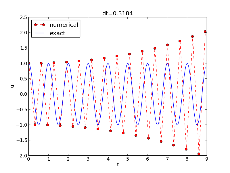
Growing, unstable solution because of a time step slightly beyond the stability limit
About the accuracy at the stability limit
An interesting question is whether the stability condition \(\Delta t < 2/\omega\) is unfortunate, or more precisely: would it be meaningful to take larger time steps to speed up computations? The answer is a clear no. At the stability limit, we have that \(\sin^{-1}\omega\Delta t/2 = \sin^{-1} 1 = \pi/2\), and therefore \(\tilde\omega = \pi/\Delta t\). (Note that the approximate formula (19) is very inaccurate for this value of \(\Delta t\) as it predicts \(\tilde\omega = 2.34/pi\), which is a 25 percent reduction.) The corresponding period of the numerical solution is \(\tilde P=2\pi/\tilde\omega = 2\Delta t\), which means that there is just one time step \(\Delta t\) between a peak (maximum) and a through (minimum) in the numerical solution. This is the shortest possible wave that can be represented in the mesh! In other words, it is not meaningful to use a larger time step than the stability limit.
Also, the error in angular frequency when \(\Delta t = 2/\omega\) is severe: Figure Numerical solution with \( Delta t \) exactly at the stability limit shows a comparison of the numerical and analytical solution with \(\omega = 2\pi\) and \(\Delta t = 2/\omega = \pi^{-1}\). Already after one period, the numerical solution has a through while the exact solution has a peak (!). The error in frequency when \(\Delta t\) is at the stability limit becomes \(\omega - \tilde\omega = \omega(1-\pi/2)\approx -0.57\omega\). The corresponding error in the period is \(P - \tilde P \approx 0.36P\). The error after \(m\) periods is then \(0.36mP\). This error has reached half a period when \(m=1/(2\cdot 0.36)\approx 1.38\), which theoretically confirms the observations in Figure Numerical solution with \( Delta t \) exactly at the stability limit that the numerical solution is a through ahead of a peak already after one and a half period. Consequently, \(\Delta t\) should be chosen much less than the stability limit to achieve meaningful numerical computations.
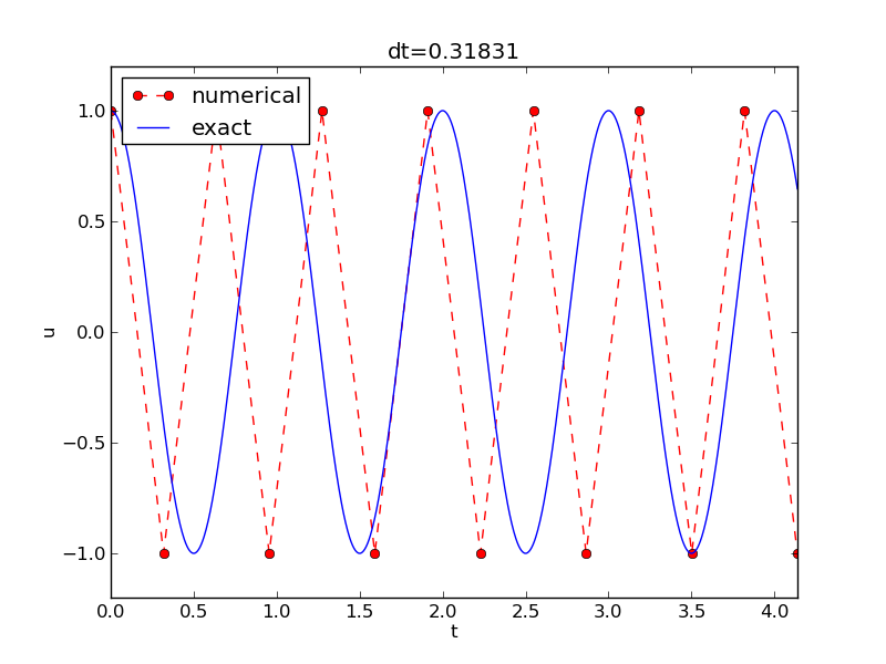
Numerical solution with \( Delta t \) exactly at the stability limit
Summary
From the accuracy and stability analysis we can draw three important conclusions:
- The key parameter in the formulas is \(p=\omega\Delta t\). The period of oscillations is \(P=2\pi/\omega\), and the number of time steps per period is \(N_P=P/\Delta t\). Therefore, \(p=\omega\Delta t = 2\pi/N_P\), showing that the critical parameter is the number of time steps per period. The smallest possible \(N_P\) is 2, showing that \(p\in (0,\pi]\).
- Provided \(p\leq 2\), the amplitude of the numerical solution is constant.
- The ratio of the numerical angular frequency and the exact one is \(\tilde\omega/\omega \approx 1 + \frac{1}{24}p^2\). The error \(\frac{1}{24}p^2\) leads to wrongly displaced peaks of the numerical solution, and the error in peak location grows linearly with time (see Exercise 1.2: Show linear growth of the phase with time).
Alternative schemes based on 1st-order equations
A standard technique for solving second-order ODEs is to rewrite them as a system of first-order ODEs and then choose a solution strategy from the vast collection of methods for first-order ODE systems. Given the second-order ODE problem
we introduce the auxiliary variable \(v=u^{\prime}\) and express the ODE problem in terms of first-order derivatives of \(u\) and \(v\):
The initial conditions become \(u(0)=I\) and \(v(0)=0\).
The Forward Euler scheme
A Forward Euler approximation to our \(2\times 2\) system of ODEs (24)-(25) becomes
or written out,
Let us briefly compare this Forward Euler method with the centered difference scheme for the second-order differential equation. We have from (28) and (29) applied at levels \(n\) and \(n-1\) that
Since from (28)
it follows that
which is very close to the centered difference scheme, but the last term is evaluated at \(t_{n-1}\) instead of \(t_n\). Rewriting, so that \(\Delta t^2\omega^2u^{n-1}\) appears alone on the right-hand side, and then dividing by \(\Delta t^2\), the new left-hand side is an approximation to \(u^{\prime\prime}\) at \(t_n\), while the right-hand side is sampled at \(t_{n-1}\). All terms should be sampled at the same mesh point, so using \(\omega^2 u^{n-1}\) instead of \(\omega^2 u^n\) points to a kind of mathematical error in the derivation of the scheme. This error turns out to be rather crucial for the accuracy of the Forward Euler method applied to vibration problems (the section Comparison of schemes has examples).
The reasoning above does not imply that the Forward Euler scheme is not correct, but more that it is almost equivalent to a second-order accurate scheme for the second-order ODE formulation, and that the error committed has to do with a wrong sampling point.
The Backward Euler scheme
A Backward Euler approximation to the ODE system is equally easy to write up in the operator notation:
This becomes a coupled system for \(u^{n+1}\) and \(v^{n+1}\):
We can compare (32)-(33) with the centered scheme (7) for the second-order differential equation. To this end, we eliminate \(v^{n+1}\) in (32) using (33) solved with respect to \(v^{n+1}\). Thereafter, we eliminate \(v^n\) using (32) solved with respect to \(v^{n+1}\) and also replacing \(n+1\) by \(n\) and \(n\) by \(n-1\). The resulting equation involving only \(u^{n+1}\), \(u^n\), and \(u^{n-1}\) can be ordered as
which has almost the same form as the centered scheme for the second-order differential equation, but the right-hand side is evaluated at \(u^{n+1}\) and not \(u^n\). This inconsistent sampling of terms has a dramatic effect on the numerical solution, as we demonstrate in the section Comparison of schemes.
The Crank-Nicolson scheme
The Crank-Nicolson scheme takes this form in the operator notation:
Writing the equations out and rearranging terms, shows that this is also a coupled system of two linear equations at each time level:
We may compare also this scheme to the centered discretization of the second-order ODE. It turns out that the Crank-Nicolson scheme is equivalent to the discretization
That is, the Crank-Nicolson is equivalent to (7) for the second-order ODE, apart from an extra term of size \(\Delta t^2\), but this is an error of the same order as in the finite difference approximation on the left-hand side of the equation anyway. The fact that the Crank-Nicolson scheme is so close to (7) makes it a much better method than the Forward or Backward Euler methods for vibration problems, as will be illustrated in the section Comparison of schemes.
Deriving (38) is a bit tricky. We start with rewriting the Crank-Nicolson equations as follows
and add the latter at the previous time level as well:
We can also rewrite (39) at the previous time level as
Inserting (40) for \(v^{n+1}\) in (39) and (41) for \(v^{n}\) in (39) yields after some reordering:
Now, \(v^n + v^{n-1}\) can be eliminated by means of (42). The result becomes
It can be shown that
meaning that (43) is an approximation to the centered scheme (7) for the second-order ODE where the sampling error in the term \(\Delta t^2\omega^2 u^n\) is of the same order as the approximation errors in the finite differences, i.e., \({\mathcal{O}(\Delta t^2)}\). The Crank-Nicolson scheme written as (43) therefore has consistent sampling of all terms at the same time point \(t_n\).
Comparison of schemes
We can easily compare methods like the ones above (and many more!) with the aid of the Odespy package. Below is a sketch of the code.
import odespy
import numpy as np

def f(u, t, w=1):
    # v, u numbering for EulerCromer to work well
    v, u = u  # u is array of length 2 holding our [v, u]
    return [-w**2*u, v]

def run_solvers_and_plot(solvers, timesteps_per_period=20,
                         num_periods=1, I=1, w=2*np.pi):
    P = 2*np.pi/w  # duration of one period
    dt = P/timesteps_per_period
    Nt = num_periods*timesteps_per_period
    T = Nt*dt
    t_mesh = np.linspace(0, T, Nt+1)

    legends = []
    for solver in solvers:
        solver.set(f_kwargs={'w': w})
        solver.set_initial_condition([0, I])
        u, t = solver.solve(t_mesh)
There is quite some more code dealing with plots also, and we refer
to the source file vib_undamped_odespy.py
for details. Observe that keyword arguments in f(u,t,w=1) can
be supplied through a solver parameter f_kwargs (dictionary of
additional keyword arguments to f).
Specification of the Forward Euler, Backward Euler, and Crank-Nicolson schemes is done like this:
solvers = [
    odespy.ForwardEuler(f),
    # Implicit methods must use Newton solver to converge
    odespy.BackwardEuler(f, nonlinear_solver='Newton'),
    odespy.CrankNicolson(f, nonlinear_solver='Newton'),
    ]
The vib_undamped_odespy.py program makes two plots of the computed
solutions with the various methods in the solvers list: one plot
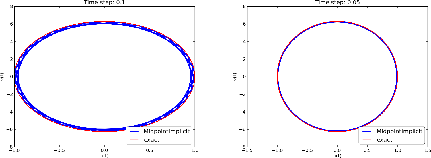
with \(u(t)\) versus \(t\), and one phase plane plot where \(v\) is
plotted against \(u\). That is, the phase plane plot is the curve
\((u(t),v(t))\) parameterized by \(t\). Analytically, \(u=I\cos(\omega t)\)
and \(v=u^{\prime}=-\omega I\sin(\omega t)\). The exact curve
\((u(t),v(t))\) is therefore an ellipse, which often looks like a circle
in a plot if the axes are automatically scaled. The important feature,
however, is that the exact curve \((u(t),v(t))\) is closed and repeats
itself for every period. Not all numerical schemes are capable of
doing that, meaning that the amplitude instead shrinks or grows with
time.
Figure Comparison of classical schemes in the phase plane for two time step values show the
results. Note that Odespy applies the label MidpointImplicit for what
we have specified as CrankNicolson in the code (CrankNicolson is
just a synonym for class MidpointImplicit in the Odespy code). The
Forward Euler scheme in Figure
Comparison of classical schemes in the phase plane for two time step values has a pronounced spiral
curve, pointing to the fact that the amplitude steadily grows, which
is also evident in Figure Comparison of solution curves for classical schemes. The
Backward Euler scheme has a similar feature, except that the spriral
goes inward and the amplitude is significantly damped. The changing
amplitude and the spiral form decreases with decreasing time step.
The Crank-Nicolson scheme looks much more accurate. In fact, these
plots tell that the Forward and Backward Euler schemes are not
suitable for solving our ODEs with oscillating solutions.
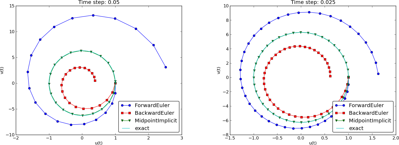
Comparison of classical schemes in the phase plane for two time step values
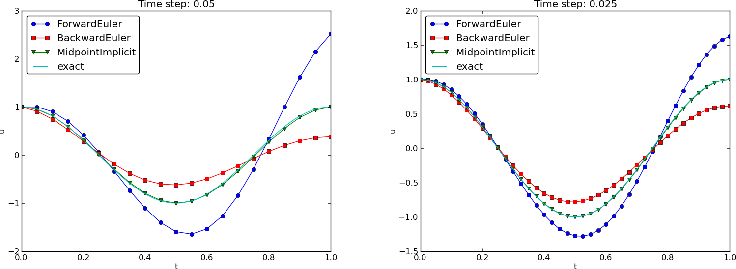
Comparison of solution curves for classical schemes
Runge-Kutta methods
We may run two other popular standard methods for first-order ODEs, the 2nd- and 4th-order Runge-Kutta methods, to see how they perform. Figures Comparison of Runge-Kutta schemes in the phase plane and Comparison of Runge-Kutta schemes show the solutions with larger \(\Delta t\) values than what was used in the previous two plots.
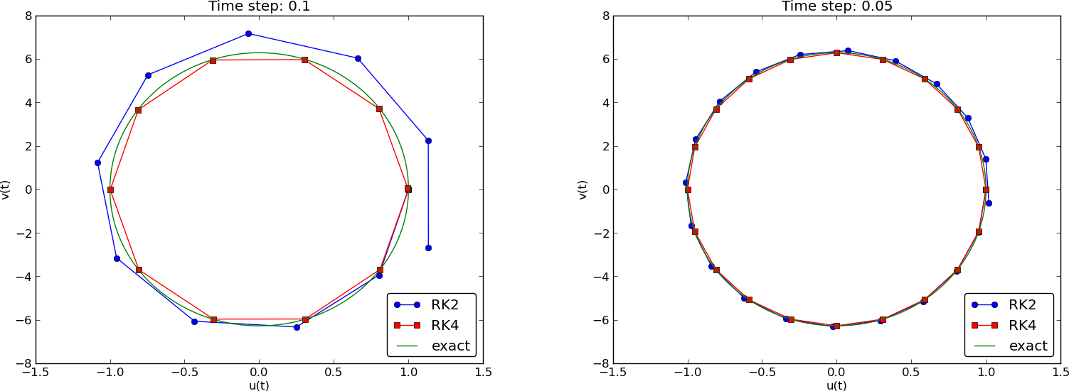
Comparison of Runge-Kutta schemes in the phase plane
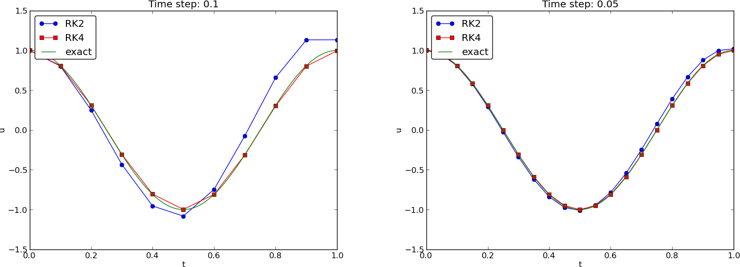
Comparison of Runge-Kutta schemes
The visual impression is that the 4th-order Runge-Kutta method is very accurate, under all circumstances in these tests, while the 2nd-order scheme suffers from amplitude errors unless the time step is very small.
The corresponding results for the Crank-Nicolson scheme are shown in Figure Long-time behavior of the Crank-Nicolson scheme in the phase plane. It is clear that the Crank-Nicolson scheme outperforms the 2nd-order Runge-Kutta method. Both schemes have the same order of accuracy \(\Oof{\Delta t^2}\), but their differences in the accuracy that matters in a real physical application is very clearly pronounced in this example. Exercise 1.13: Investigate the amplitude errors of many solvers invites you to investigate how the amplitude is computed by a series of famous methods for first-order ODEs.
Long-time behavior of the Crank-Nicolson scheme in the phase plane
Analysis of the Forward Euler scheme
We may try to find exact solutions of the discrete equations (28)-(29) in the Forward Euler method to better understand why this otherwise useful method has so bad performance for vibration ODEs. An “ansatz” for the solution of the discrete equations is
where \(q\) and \(A\) are scalars to be determined. We could have used a complex exponential form \(e^{i\tilde\omega n\Delta t}\) since we get oscillatory solutions, but the oscillations grow in the Forward Euler method, so the numerical frequency \(\tilde\omega\) will be complex anyway (producing an exponentially growing amplitude). Therefore, it is easier to just work with potentially complex \(A\) and \(q\) as introduced above.
The Forward Euler scheme leads to
We can easily eliminate \(A\), get \(q^2 + \omega^2=0\), and solve for
which gives
We shall take the real part of \(A^n\) as the solution. The two values of \(A\) are complex conjugates, and the real part of \(A^n\) will be the same for both roots. This is easy to realize if we rewrite the complex numbers in polar form, which is also convenient for further analysis and understanding. The polar form \(re^{i\theta}\) of a complex number \(x+iy\) has \(r=\sqrt{x^2+y^2}\) and \(\theta = \tan^{-1}(y/x)\). Hence, the polar form of the two values for \(A\) becomes
Now it is very easy to compute \(A^n\):
Since \(\cos (\theta n) = \cos (-\theta n)\), the real parts of the two numbers become the same. We therefore continue with the solution that has the plus sign.
The general solution is \(u^n = CA^n\), where \(C\) is a constant determined from the initial condition: \(u^0=C=I\). We have \(u^n=IA^n\) and \(v^n=qIA^n\). The final solutions are just the real part of the expressions in polar form:
The expression \((1+\omega^2\Delta t^2)^{n/2}\) causes growth of
the amplitude, since a number greater than one is raised to a positive
exponent \(n/2\). We can develop a series expression to better understand
the formula for the amplitude. Introducing \(p=\omega\Delta t\) as the
key variable and using sympy gives
>>> from sympy import *
>>> p = symbols('p', real=True)
>>> n = symbols('n', integer=True, positive=True)
>>> amplitude = (1 + p**2)**(n/2)
>>> amplitude.series(p, 0, 4)
1 + n*p**2/2 + O(p**4)
The amplitude goes like \(1 + \frac{1}{2} n\omega^2\Delta t^2\), clearly growing linearly in time (with \(n\)).
We can also investigate the error in the angular frequency by a series expansion:
>>> n*atan(p).series(p, 0, 4)
n*(p - p**3/3 + O(p**4))
This means that the solution for \(u^n\) can be written as
The error in the angular frequency is of the same order as in the scheme (7) for the second-order ODE, but the error in the amplitude is severe.
Energy considerations
The observations of various methods in the previous section can be better interpreted if we compute a quantity reflecting the total energy of the system. It turns out that this quantity,
is constant for all \(t\). Checking that \(E(t)\) really remains constant brings evidence that the numerical computations are sound. It turns out that \(E\) is proportional to the mechanical energy in the system. Conservation of energy is much used to check numerical simulations, so it is well invested time to dive into this subject.
Derivation of the energy expression
We start out with multiplying
by \(u^{\prime}\) and integrating from \(0\) to \(T\):
Observing that
we get
where we have introduced
The important result from this derivation is that the total energy is constant:
Energy of the exact solution
Analytically, we have \(u(t)=I\cos\omega t\), if \(u(0)=I\) and \(u^{\prime}(0)=0\), so we can easily check the energy evolution and confirm that \(E(t)\) is constant:
Growth of energy in the Forward Euler scheme
The energy at time level \(n+1\) in the Forward Euler scheme can easily be shown to increase:
An error measure based on energy
The constant energy is well expressed by its initial value \(E(0)\), so that the error in mechanical energy can be computed as a mesh function by
where
if \(u(0)=I\) and \(u^{\prime}(0)=V\). Note that we have used a centered approximation to \(u^{\prime}\): \(u^{\prime}(t_n)\approx [D_{2t}u]^n\).
A useful norm of the mesh function \(e_E^n\) for the discrete mechanical energy can be the maximum absolute value of \(e_E^n\):
Alternatively, we can compute other norms involving integration over all mesh points, but we are often interested in worst case deviation of the energy, and then the maximum value is of particular relevance.
A vectorized Python implementation of \(e_E^n\) takes the form
# import numpy as np and compute u, t
dt = t[1]-t[0]
E = 0.5*((u[2:] - u[:-2])/(2*dt))**2 + 0.5*w**2*u[1:-1]**2
E0 = 0.5*V**2 + 0.5**w**2*I**2
e_E = E - E0
e_E_norm = np.abs(e_E).max()
The convergence rates of the quantity e_E_norm can be used for
verification. The value of e_E_norm is also useful for comparing
schemes through their ability to preserve energy. Below is a table
demonstrating the relative error in total energy for various schemes
(computed by the vib_undamped_odespy.py program). The test problem is
\(u^{\prime\prime} + 4\pi^2 u =0\) with \(u(0)=1\) and \(u'(0)=0\), so the
period is 1 and \(E(t)\approx 4.93\). We clearly see that the
Crank-Nicolson and the Runge-Kutta schemes are superior to the Forward
and Backward Euler schemes already after one period.
| Method | \(T\) | \(\Delta t\) | \(\max \left\vert e_E^n\right\vert/e_E^0\) |
|---|---|---|---|
| Forward Euler | \(1\) | \(0.025\) | \(1.678\cdot 10^{0}\) |
| Backward Euler | \(1\) | \(0.025\) | \(6.235\cdot 10^{-1}\) |
| Crank-Nicolson | \(1\) | \(0.025\) | \(1.221\cdot 10^{-2}\) |
| Runge-Kutta 2nd-order | \(1\) | \(0.025\) | \(6.076\cdot 10^{-3}\) |
| Runge-Kutta 4th-order | \(1\) | \(0.025\) | \(8.214\cdot 10^{-3}\) |
However, after 10 periods, the picture is much more dramatic:
| Method | \(T\) | \(\Delta t\) | \(\max \left\vert e_E^n\right\vert/e_E^0\) |
|---|---|---|---|
| Forward Euler | \(10\) | \(0.025\) | \(1.788\cdot 10^{4}\) |
| Backward Euler | \(10\) | \(0.025\) | \(1.000\cdot 10^{0}\) |
| Crank-Nicolson | \(10\) | \(0.025\) | \(1.221\cdot 10^{-2}\) |
| Runge-Kutta 2nd-order | \(10\) | \(0.025\) | \(6.250\cdot 10^{-2}\) |
| Runge-Kutta 4th-order | \(10\) | \(0.025\) | \(8.288\cdot 10^{-3}\) |
The Runge-Kutta and Crank-Nicolson methods hardly change their energy error with \(T\), while the error in the Forward Euler method grows to huge levels and a relative error of 1 in the Backward Euler method points to \(E(t)\rightarrow 0\) as \(t\) grows large.
Running multiple values of \(\Delta t\), we can get some insight into the convergence of the energy error:
| Method | \(T\) | \(\Delta t\) | \(\max \left\vert e_E^n\right\vert/e_E^0\) |
|---|---|---|---|
| Forward Euler | \(10\) | \(0.05\) | \(1.120\cdot 10^{8}\) |
| Forward Euler | \(10\) | \(0.025\) | \(1.788\cdot 10^{4}\) |
| Forward Euler | \(10\) | \(0.0125\) | \(1.374\cdot 10^{2}\) |
| Backward Euler | \(10\) | \(0.05\) | \(1.000\cdot 10^{0}\) |
| Backward Euler | \(10\) | \(0.025\) | \(1.000\cdot 10^{0}\) |
| Backward Euler | \(10\) | \(0.0125\) | \(9.928\cdot 10^{-1}\) |
| Crank-Nicolson | \(10\) | \(0.05\) | \(4.756\cdot 10^{-2}\) |
| Crank-Nicolson | \(10\) | \(0.025\) | \(1.221\cdot 10^{-2}\) |
| Crank-Nicolson | \(10\) | \(0.0125\) | \(3.125\cdot 10^{-3}\) |
| Runge-Kutta 2nd-order | \(10\) | \(0.05\) | \(6.152\cdot 10^{-1}\) |
| Runge-Kutta 2nd-order | \(10\) | \(0.025\) | \(6.250\cdot 10^{-2}\) |
| Runge-Kutta 2nd-order | \(10\) | \(0.0125\) | \(7.631\cdot 10^{-3}\) |
| Runge-Kutta 4th-order | \(10\) | \(0.05\) | \(3.510\cdot 10^{-2}\) |
| Runge-Kutta 4th-order | \(10\) | \(0.025\) | \(8.288\cdot 10^{-3}\) |
| Runge-Kutta 4th-order | \(10\) | \(0.0125\) | \(2.058\cdot 10^{-3}\) |
A striking fact from this table is that the error of the Forward Euler method is reduced by the same factor as \(\Delta t\) is reduced by, while the error in the Crank-Nicolson method has a reduction proportional to \(\Delta t^2\) (we cannot say anything for the Backward Euler method). However, for the RK2 method, halving \(\Delta t\) reduces the error by almost a factor of 10 (!), and for the RK4 method the reduction seems proportional to \(\Delta t^2\) only (and the trend is confirmed by running smaller time steps, so for \(\Delta t = 3.9\cdot 10^{-4}\) the relative error of RK2 is a factor 10 smaller than that of RK4!).
The Euler-Cromer method
While the Runge-Kutta methods and the Crank-Nicolson scheme work well for the vibration equation modeled as a first-order ODE system, both were inferior to the straightforward centered difference scheme for the second-order equation \(u^{\prime\prime}+\omega^2u=0\). However, there is a similarly successful scheme available for the first-order system \(u^{\prime}=v\), \(v^{\prime}=-\omega^2u\), to be presented below. The ideas of the scheme and their further developments have become very popular in particle and rigid body dynamics and hence widely used by physicists.
Forward-backward discretization
The idea is to apply a Forward Euler discretization to the first equation and a Backward Euler discretization to the second. In operator notation this is stated as
We can write out the formulas and collect the unknowns on the left-hand side:
We realize that after \(u^{n+1}\) has been computed from (52), it may be used directly in (53) to compute \(v^{n+1}\).
In physics, it is more common to update the \(v\) equation first, with a forward difference, and thereafter the \(u\) equation, with a backward difference that applies the most recently computed \(v\) value:
The advantage of ordering the ODEs as in (54)-(55) becomes evident when considering complicated models. Such models are included if we write our vibration ODE more generally as
We can rewrite this second-order ODE as two first-order ODEs,
This rewrite allows the following scheme to be used:
We realize that the first update works well with any \(g\) since old values \(u^n\) and \(v^n\) are used. Switching the equations would demand \(u^{n+1}\) and \(v^{n+1}\) values in \(g\) and result in nonlinear algebraic equations to be solved at each time level.
The scheme (54)-(55) goes under several names: forward-backward scheme, semi-implicit Euler method, semi-explicit Euler, symplectic Euler, Newton-Stoermer-Verlet, and Euler-Cromer. We shall stick to the latter name. Since both time discretizations are based on first-order difference approximation, one may think that the scheme is only of first-order, but this is not true: the use of a forward and then a backward difference make errors cancel so that the overall error in the scheme is \(\Oof{\Delta t^2}\). This is explained below.
How does the Euler-Cromer method preserve the total energy? We may run the example from the section An error measure based on energy:
| Method | \(T\) | \(\Delta t\) | \(\max \left\vert e_E^n\right\vert/e_E^0\) |
|---|---|---|---|
| Euler-Cromer | \(10\) | \(0.05\) | \(2.530\cdot 10^{-2}\) |
| Euler-Cromer | \(10\) | \(0.025\) | \(6.206\cdot 10^{-3}\) |
| Euler-Cromer | \(10\) | \(0.0125\) | \(1.544\cdot 10^{-3}\) |
The relative error in the total energy decreases as \(\Delta t^2\), and the error level is slightly lower than for the Crank-Nicolson and Runge-Kutta methods.
Equivalence with the scheme for the second-order ODE
We shall now show that the Euler-Cromer scheme for the system of first-order equations is equivalent to the centered finite difference method for the second-order vibration ODE (!).
We may eliminate the \(v^n\) variable from (52)-(53) or (54)-(55). The \(v^{n+1}\) term in (54) can be eliminated from (55):
The \(v^{n}\) quantity can be expressed by \(u^n\) and \(u^{n-1}\) using (55):
and when this is inserted in (56) we get
which is nothing but the centered scheme (7)! The two seemingly different numerical methods are mathematically equivalent. Consequently, the previous analysis of (7) also applies to the Euler-Cromer method. In particular, the amplitude is constant, given that the stability criterion is fulfilled, but there is always an angular frequency error (19). Exercise 1.18: Analysis of the Euler-Cromer scheme gives guidance on how to derive the exact discrete solution of the two equations in the Euler-Cromer method.
Although the Euler-Cromer scheme and the method (7) are equivalent, there could be differences in the way they handle the initial conditions. Let is look into this topic. The initial condition \(u^{\prime}=0\) means \(u^{\prime}=v=0\). From (54) we get
and from (55) it follows that
When we previously used a centered approximation of \(u^{\prime}(0)=0\) combined with the discretization (7) of the second-order ODE, we got a slightly different result: \(u^1=u^0 - \frac{1}{2}\omega^2\Delta t^2 u^0\). The difference is \(\frac{1}{2}\omega^2\Delta t^2 u^0\), which is of second order in \(\Delta t\), seemingly consistent with the overall error in the scheme for the differential equation model.
A different view can also be taken. If we approximate \(u^{\prime}(0)=0\) by a backward difference, \((u^0-u^{-1})/\Delta t =0\), we get \(u^{-1}=u^0\), and when combined with (7), it results in \(u^1=u^0 - \omega^2\Delta t^2 u^0\). This means that the Euler-Cromer method based on (55)-(54) corresponds to using only a first-order approximation to the initial condition in the method from the section A centered finite difference scheme.
Correspondingly, using the formulation (52)-(53) with \(v^n=0\) leads to \(u^1=u^0\), which can be interpreted as using a forward difference approximation for the initial condition \(u^{\prime}(0)=0\). Both Euler-Cromer formulations lead to slightly different values for \(u^1\) compared to the method in the section A centered finite difference scheme. The error is \(\frac{1}{2}\omega^2\Delta t^2 u^0\).
Implementation
Solver function
The function below, found in vib_undamped_EulerCromer.py, implements the Euler-Cromer scheme (54)-(55):
import numpy as np

def solver(I, w, dt, T):
    """
    Solve v' = - w**2*u, u'=v for t in (0,T], u(0)=I and v(0)=0,
    by an Euler-Cromer method.
    """
    dt = float(dt)
    Nt = int(round(T/dt))
    u = np.zeros(Nt+1)
    v = np.zeros(Nt+1)
    t = np.linspace(0, Nt*dt, Nt+1)

    v[0] = 0
    u[0] = I
    for n in range(0, Nt):
        v[n+1] = v[n] - dt*w**2*u[n]
        u[n+1] = u[n] + dt*v[n+1]
    return u, v, t
Verification
Since the Euler-Cromer scheme is equivalent to the finite difference
method for the second-order ODE \(u^{\prime\prime}+\omega^2u=0\) (see the section Equivalence with the scheme for the second-order ODE), the performance of the above
solver function is the same as for the solver function in the section Implementation. The only difference is the formula for the first time
step, as discussed above. This deviation in the Euler-Cromer scheme
means that the discrete solution listed in the section Exact discrete solution is not a solution of the Euler-Cromer
scheme!
To verify the implementation of the Euler-Cromer method we can adjust
v[1] so that the computer-generated values can be compared with the
formula (20) from in the section Exact discrete solution. This adjustment is done in an alternative
solver function, solver_ic_fix in vib_EulerCromer.py. Since we now
have an exact solution of the discrete equations available, we can
write a test function test_solver for checking the equality of
computed values with the formula (20):
def test_solver():
    """
    Test solver with fixed initial condition against
    equivalent scheme for the 2nd-order ODE u'' + u = 0.
    """
    I = 1.2; w = 2.0; T = 5
    dt = 2/w  # longest possible time step
    u, v, t = solver_ic_fix(I, w, dt, T)
    from vib_undamped import solver as solver2  # 2nd-order ODE
    u2, t2 = solver2(I, w, dt, T)
    error = np.abs(u - u2).max()
    tol = 1E-14
    assert error < tol
Another function, demo, visualizes the difference between the
Euler-Cromer scheme and the scheme (7) for the
second-oder ODE, arising from the mismatch in the first time level.
Using Odespy
The Euler-Cromer method is also available in the Odespy package. The
important thing to remember, when using this implementation, is that
we must order the unknowns as \(v\) and \(u\), so the u vector at each
time level consists of the velocity \(v\) as first component and the
displacement \(u\) as second component:
# Define ODE
def f(u, t, w=1):
    v, u = u
    return [-w**2*u, v]

# Initialize solver
I = 1
w = 2*np.pi
import odespy
solver = odespy.EulerCromer(f, f_kwargs={'w': w})
solver.set_initial_condition([0, I])

# Compute time mesh
P = 2*np.pi/w  # duration of one period
dt = P/timesteps_per_period
Nt = num_periods*timesteps_per_period
T = Nt*dt
import numpy as np
t_mesh = np.linspace(0, T, Nt+1)

# Solve ODE
u, t = solver.solve(t_mesh)
u = u[:,1]  # Extract displacement
Convergence rates
We may use the convergence_rates function in the file
vib_undamped.py to investigate the convergence rate of the
Euler-Cromer method, see the convergence_rate function in the file
vib_undamped_EulerCromer.py. Since we could eliminate \(v\) to get a
scheme for \(u\) that is equivalent to the finite difference method for
the second-order equation in \(u\), we would expect the convergence
rates to be the same, i.e., \(\mathcal{O}(\Delta t^2)\). However,
measuring the convergence rate of \(u\) in the Euler-Cromer scheme shows
that it is \(\mathcal{O}(\Delta t)\)! Adjusting the initial condition
does not change the rate. Adjusting \(\omega\), as outlined in the section The error in the numerical frequency, gives a 4th-order method there, while
there is no increase in the measured rate in the Euler-Cromer
scheme. It is obvious that the Euler-Cromer scheme is dramatically
much better than the two other first-order methods, Forward Euler and
Backward Euler, but this is not reflected in the convergence rate of
\(u\).
The Stoermer-Verlet algorithm
Another very popular algorithm for vibration problems, especially for long time simulations, is the Stoermer-Verlet algorithm. It has become the method among physicists for molecular simulations as well as particle and rigid body dynamics.
The method can be derived by applying the Euler-Cromer idea twice, in a symmetric fashion, during the interval \([t_n,t_{n+1}]\):
- solve \(v^{\prime}=-\omega u\) by a Forward Euler step in \([t_n,t_{n+\frac{1}{2}}]\)
- solve \(u^{\prime}=v\) by a Backward Euler step in \([t_n,t_{n+\frac{1}{2}}]\)
- solve \(u^{\prime}=v\) by a Forward Euler step in \([t_{n+\frac{1}{2}}, t_{n+1}]\)
- solve \(v^{\prime}=-\omega u\) by a Backward Euler step in \([t_{n+\frac{1}{2}}, t_{n+1}]\)
With mathematics,
The two steps in the middle can be combined to
and consequently
Writing the last equation as \(v^n = v^{n-\frac{1}{2}} - \frac{1}{2}\Delta t\omega^2 u^n\) and using this \(v^n\) in the first equation gives \(v^{n+\frac{1}{2}} = v^{n-\frac{1}{2}} - \Delta t\omega^2 u^n\), and the scheme can be written as two steps:
which is nothing but straightforward centered differences for the \(2\times 2\) ODE system on a staggered mesh, see the section The Euler-Cromer scheme on a staggered mesh. We have thus seen that four different reasonings (discretizing \(u^{\prime\prime}+\omega^2 u\) directly, using Euler-Cromer, using Stoermer-Verlet, and using centered differences for the \(2times 2\) system on a staggered mesh) all end up with the same equations! The main difference is that the traditional Euler-Cromer displays first-order convergence in \(\Delta t\) (due to less symmetry in the way \(u\) and \(v\) are treated) while the others are \({\mathcal{O}(\Delta t^2)}\) schemes.
The most numerical stable scheme, with respect to accumulation of rounding errors, is (61)-(62). It has, according to [Ref04], better properties in this regard than the direct scheme for the second-order ODE.
Staggered mesh
A more intuitive discretization than the Euler-Cromer method, yet equivalent, employs solely centered differences in a natural way for the \(2\times 2\) first-order ODE system. The scheme is in fact fully equivalent to the second-order scheme for \(u''+\omega u=0\), also for the first time step. Such a scheme needs to operate on a staggered mesh in time. Staggered meshes are very popular in many physical application, maybe foremost fluid dynamics and electromagnetics, so the topic is important to learn.
The Euler-Cromer scheme on a staggered mesh
In a staggered mesh, the unknowns are sought at different points in the mesh. Specifically, \(u\) is sought at integer time points \(t_n\) and \(v\) is sought at \(t_{n+1/2}\) between two \(u\) points. The unknowns are then \(u^1, v^{3/2}, u^2, v^{5/2}\), and so on. We typically use the notation \(u^n\) and \(v^{n+\frac{1}{2}}\) for the two unknown mesh functions. Figure Examples on mesh functions on a staggered mesh in time presents a graphical sketch of two mesh functions \(u\) and \(v\) on a staggered mesh.
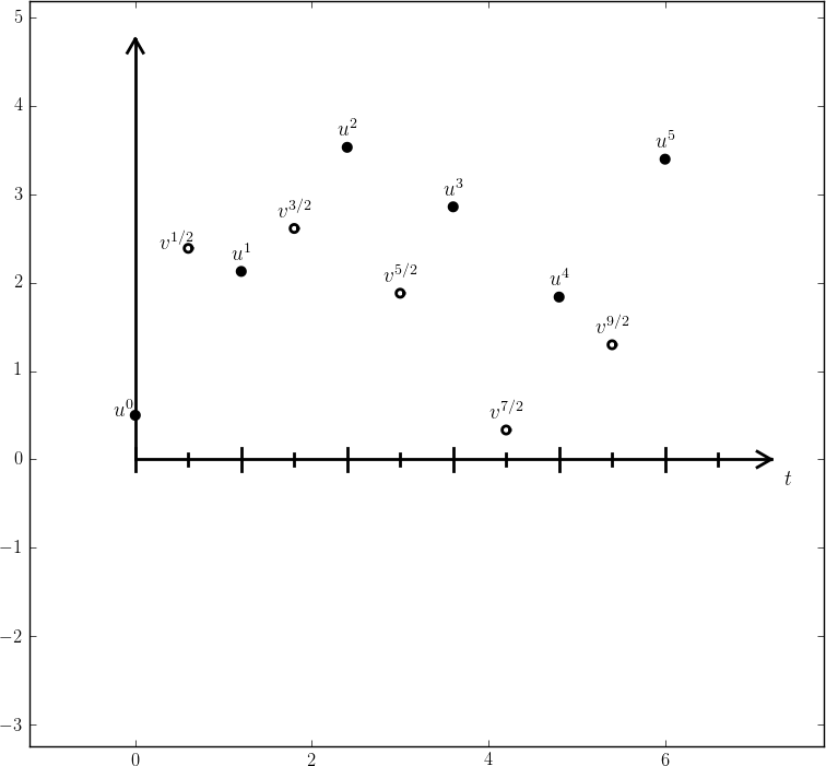
Examples on mesh functions on a staggered mesh in time
On a staggered mesh it is natural to use centered difference approximations, expressed in operator notation as
or if we switch the sequence of the equations:
Writing out the formulas gives
We can eliminate the \(v\) values and get back the centered scheme based on the second-order differential equation \(u^{\prime\prime} +\omega^2 u = 0\), so all these three schemes are equivalent. However, they differ somewhat in the treatment of the initial conditions.
Suppose we have \(u(0)=I\) and \(u'(0)=v(0)=0\) as mathematical initial conditions. This means \(u^0=I\) and
Using the discretized equation (67) for \(n=0\) yields
and eliminating \(v^{-\frac{1}{2}} =- v^{\frac{1}{2}}\) results in
and
which is exactly the same equation for \(u^1\) as we had in the centered scheme based on the second-order differential equation (and hence corresponds to a centered difference approximation of the initial condition for \(u'(0)\)). The conclusion is that a staggered mesh is fully equivalent with that scheme, while the forward-backward version gives a slight deviation in the computation of \(u^1\).
We can redo the derivation of the initial conditions when \(u'(0)=V\):
Using this \(v^{-\frac{1}{2}}\) in
then gives \(v^\frac{1}{2} = V - \frac{1}{2}\Delta t\omega^2 I\). The general initial conditions are therefore
Implementation of the scheme on a staggered mesh
The algorithm goes like this:
Implementation with integer indices
Translating the schemes (68)
and (67) to computer code
faces the problem of how to store and access \(v^{n+\frac{1}{2}}\),
since arrays only allow integer indices with base 0.
We must then introduce a convention: \(v^{1+\frac{1}{2}}\) is stored
in v[n] while \(v^{1-\frac{1}{2}}\) is stored in v[n-1].
We can then write the algorithm in Python as
def solver(I, w, dt, T):
    dt = float(dt)
    Nt = int(round(T/dt))
    u = zeros(Nt+1)
    v = zeros(Nt+1)
    t = linspace(0, Nt*dt, Nt+1)  # mesh for u
    t_v = t + dt/2                # mesh for v

    u[0] = I
    v[0] = 0 - 0.5*dt*w**2*u[0]
    for n in range(1, Nt+1):
        u[n] = u[n-1] + dt*v[n-1]
        v[n] = v[n-1] - dt*w**2*u[n]
    return u, t, v, t_v
Note that \(u\) and \(v\) are returned together with the mesh points such
that the complete mesh function for \(u\) is described by u and t,
while v and t_v represent the mesh function for \(v\).
Implementation with half-integer indices
~~~~~~~~~~~~~~~~~~~~~~~~~~~~~~~~~~~~~~~~
Some prefer to see a closer relationship between the code and
the mathematics for the quantities with half-integer indices.
For example, we would like to replace the updating equation for
v[n] by
v[n+half] = v[n-half] - dt*w**2*u[n]
This is easy to do if we could be sure that n+half means n and
n-half means n-1. A possible solution is to define half as a
special object such that an integer plus half results in the integer,
while an integer minus half equals the integer minus 1.
A simple Python class may realize the half object:
class HalfInt:
    def __radd__(self, other):
        return other

    def __rsub__(self, other):
        return other - 1

half = HalfInt()
The __radd__ function is invoked for all expressions n+half
(“right add” with self as half and other as n). Similarly,
the __rsub__ function is invoked for n-half and results in n-1.
Using the half object, we can implement the algorithms in an even
more readable way:
def solver(I, w, dt, T):
    """
    Solve u'=v, v' = - w**2*u for t in (0,T], u(0)=I and v(0)=0,
    by a central finite difference method with time step dt on
    a staggered mesh with v as unknown at (i+1/2)*dt time points.
    """
    dt = float(dt)
    Nt = int(round(T/dt))
    u = zeros(Nt+1)
    v = zeros(Nt+1)
    t = linspace(0, Nt*dt, Nt+1)  # mesh for u
    t_v = t + dt/2                # mesh for v

    u[0] = I
    v[0+half] = 0 - 0.5*dt*w**2*u[0]
    for n in range(1, Nt+1):
        u[n] = u[n-1] + dt*v[n-half]
        v[n+half] = v[n-half] - dt*w**2*u[n]
    return u, t, v[:-1], t_v[:-1]
Verification of this code is easy as we can just compare the computed
u with the u produced by the solver function in
vib_undamped.py (which solves \(u''+\omega^2u=0\) directly). The
values should coincide to machine precision since the two numerical
methods are mathematically equivalent. We refer to the file
vib_undamped_staggered.py
for the details of a unit test (test_staggered) that checks this property.
Exercises and Problems
Problem 1.1: Use linear/quadratic functions for verification
Consider the ODE problem
a) Discretize this equation according to \([D_tD_t u + \omega^2 u = f]^n\) and derive the equation for the first time step (\(u^1\)).
b) For verification purposes, we use the method of manufactured solutions (MMS) with the choice of \({u_{\small\mbox{e}}}(t)= ct+d\). Find restrictions on \(c\) and \(d\) from the initial conditions. Compute the corresponding source term \(f\). Show that \([D_tD_t t]^n=0\) and use the fact that the \(D_tD_t\) operator is linear, \([D_tD_t (ct+d)]^n = c[D_tD_t t]^n + [D_tD_t d]^n = 0\), to show that \({u_{\small\mbox{e}}}\) is also a perfect solution of the discrete equations.
c)
Use sympy to do the symbolic calculations above. Here is a
sketch of the program vib_undamped_verify_mms.py:
import sympy as sym
V, t, I, w, dt = sym.symbols('V t I w dt')  # global symbols
f = None  # global variable for the source term in the ODE

def ode_source_term(u):
    """Return the terms in the ODE that the source term
    must balance, here u'' + w**2*u.
    u is symbolic Python function of t."""
    return sym.diff(u(t), t, t) + w**2*u(t)

def residual_discrete_eq(u):
    """Return the residual of the discrete eq. with u inserted."""
    R = ...
    return sym.simplify(R)

def residual_discrete_eq_step1(u):
    """Return the residual of the discrete eq. at the first
    step with u inserted."""
    R = ...
    return sym.simplify(R)

def DtDt(u, dt):
    """Return 2nd-order finite difference for u_tt.
    u is a symbolic Python function of t.
    """
    return ...

def main(u):
    """
    Given some chosen solution u (as a function of t, implemented
    as a Python function), use the method of manufactured solutions
    to compute the source term f, and check if u also solves
    the discrete equations.
    """
    print '=== Testing exact solution: %s ===' % u
    print "Initial conditions u(0)=%s, u'(0)=%s:" % \
          (u(t).subs(t, 0), sym.diff(u(t), t).subs(t, 0))

    # Method of manufactured solution requires fitting f
    global f  # source term in the ODE
    f = sym.simplify(ode_lhs(u))

    # Residual in discrete equations (should be 0)
    print 'residual step1:', residual_discrete_eq_step1(u)
    print 'residual:', residual_discrete_eq(u)

def linear():
    main(lambda t: V*t + I)

if __name__ == '__main__':
    linear()
Fill in the various functions such that the calls in the main
function works.
d)
The purpose now is to choose a quadratic function
\({u_{\small\mbox{e}}} = bt^2 + ct + d\) as exact solution. Extend the sympy
code above with a function quadratic for fitting f and checking
if the discrete equations are fulfilled. (The function is very similar
to linear.)
e) Will a polynomial of degree three fulfill the discrete equations?
f)
Implement a solver function for computing the numerical
solution of this problem.
g)
Write a test function for checking that the quadratic solution
is computed correctly (to machine precision, but the
round-off errors accumulate and increase with \(T\)) by the solver
function.
Filename: vib_undamped_verify_mms.
Exercise 1.2: Show linear growth of the phase with time
Consider an exact solution \(I\cos (\omega t)\) and an approximation \(I\cos(\tilde\omega t)\). Define the phase error as the time lag between the peak \(I\) in the exact solution and the corresponding peak in the approximation after \(m\) periods of oscillations. Show that this phase error is linear in \(m\).
Filename: vib_phase_error_growth.
Exercise 1.3: Improve the accuracy by adjusting the frequency
According to (19), the numerical
frequency deviates from the exact frequency by a (dominating) amount
\(\omega^3\Delta t^2/24 >0\). Replace the w parameter in the algorithm
in the solver function in vib_undamped.py by w*(1 -
(1./24)*w**2*dt**2 and test how this adjustment in the numerical
algorithm improves the accuracy (use \(\Delta t =0.1\) and simulate
for 80 periods, with and without adjustment of \(\omega\)).
Filename: vib_adjust_w.
Exercise 1.4: See if adaptive methods improve the phase error
Adaptive methods for solving ODEs aim at adjusting \(\Delta t\) such
that the error is within a user-prescribed tolerance. Implement the
equation \(u^{\prime\prime}+u=0\) in the Odespy
software. Use the example on adaptive
schemes
in [Ref02]. Run the scheme with a very low
tolerance (say \(10^{-14}\)) and for a long time, check the number of
time points in the solver’s mesh (len(solver.t_all)), and compare
the phase error with that produced by the simple finite difference
method from the section A centered finite difference scheme with the same number of (equally
spaced) mesh points. The question is whether it pays off to use an
adaptive solver or if equally many points with a simple method gives
about the same accuracy.
Filename: vib_undamped_adaptive.
Exercise 1.5: Use a Taylor polynomial to compute \(u^1\)
As an alternative to computing \(u^1\) by (8), one can use a Taylor polynomial with three terms:
With \(u^{\prime\prime}=-\omega^2 u\) and \(u^{\prime}(0)=0\), show that this method also leads to (8). Generalize the condition on \(u^{\prime}(0)\) to be \(u^{\prime}(0)=V\) and compute \(u^1\) in this case with both methods.
Filename: vib_first_step.
Problem 1.6: Derive and investigate the velocity Verlet method
The velocity Verlet method for \(u^{\prime\prime} + \omega^2u=0\) is based on the following ideas:
- step \(u\) forward from \(t_n\) to \(t_{n+1}\) using a three-term Taylor series,
- replace \(u^{\prime\prime}\) by \(-\omega^2u\)
- discretize \(v^{\prime}=-\omega^2u\) by a Crank-Nicolson method.
Derive the scheme, implement it, and determine empirically the convergence rate.
Problem 1.7: Find the minimal resolution of an oscillatory function
Sketch the function on a given mesh which has the highest possible frequency. That is, this oscillatory “cos-like” function has its maxima and minima at every two grid points. Find an expression for the frequency of this function, and use the result to find the largest relevant value of \(\omega\Delta t\) when \(\omega\) is the frequency of an oscillating function and \(\Delta t\) is the mesh spacing.
Filename: vib_largest_wdt.
Exercise 1.8: Visualize the accuracy of finite differences for a cosine function
We introduce the error fraction
to measure the error in the finite difference approximation \(D_tD_tu\) to \(u^{\prime\prime}\). Compute \(E\) for the specific choice of a cosine/sine function of the form \(u=\exp{(i\omega t)}\) and show that
Plot \(E\) as a function of \(p=\omega\Delta t\). The relevant
values of \(p\) are \([0,\pi]\) (see Problem 1.7: Find the minimal resolution of an oscillatory function
for why \(p>\pi\) does not make sense).
The deviation of the curve from unity visualizes the error in the
approximation. Also expand \(E\) as a Taylor polynomial in \(p\) up to
fourth degree (use, e.g., sympy).
Filename: vib_plot_fd_exp_error.
Exercise 1.9: Verify convergence rates of the error in energy
We consider the ODE problem \(u^{\prime\prime} + \omega^2u=0\), \(u(0)=I\), \(u^{\prime}(0)=V\), for \(t\in (0,T]\). The total energy of the solution \(E(t)=\frac{1}{2}(u^{\prime})^2 + \frac{1}{2}\omega^2 u^2\) should stay constant. The error in energy can be computed as explained in the section Energy considerations.
Make a test function in a separate file, where code from
vib_undamped.py is imported, but the convergence_rates and
test_convergence_rates functions are copied and modified to also
incorporate computations of the error in energy and the convergence
rate of this error. The expected rate is 2, just as for the solution
itself.
Filename: test_error_conv.
Exercise 1.10: Use linear/quadratic functions for verification
This exercise is a generalization of Problem 1.1: Use linear/quadratic functions for verification to the extended model problem
(71) where the damping term is either linear or quadratic.
Solve the various subproblems and see how the results and problem
settings change with the generalized ODE in case of linear or
quadratic damping. By modifying the code from Problem 1.1: Use linear/quadratic functions for verification, sympy will do most
of the work required to analyze the generalized problem.
Filename: vib_verify_mms.
Exercise 1.11: Use an exact discrete solution for verification
Write a test function in a separate file
that employs the exact discrete solution
(20) to verify the implementation of the
solver function in the file vib_undamped.py.
Filename: test_vib_undamped_exact_discrete_sol.
Exercise 1.12: Use analytical solution for convergence rate tests
The purpose of this exercise is to perform convergence tests of the
problem (71) when \(s(u)=cu\), \(F(t)=A\sin\phi t\) and there
is no damping. Find the complete analytical solution to the problem
in this case (most textbooks on mechanics or ordinary differential
equations list the various elements you need to write down the exact
solution, or you can use symbolic tools like sympy or wolframalpha.com).
Modify the convergence_rate function from the
vib_undamped.py program to perform experiments with the extended
model. Verify that the error is of order \(\Delta t^2\).
Filename: vib_conv_rate.
Exercise 1.13: Investigate the amplitude errors of many solvers
Use the program vib_undamped_odespy.py from the section Comparison of schemes (utilize the function amplitudes) to investigate
how well famous methods for 1st-order ODEs can preserve the amplitude of \(u\) in undamped
oscillations. Test, for example, the 3rd- and 4th-order Runge-Kutta
methods (RK3, RK4), the Crank-Nicolson method (CrankNicolson),
the 2nd- and 3rd-order Adams-Bashforth methods (AdamsBashforth2,
AdamsBashforth3), and a 2nd-order Backwards scheme
(Backward2Step). The relevant governing equations are listed in
the beginning of the section Alternative schemes based on 1st-order equations.
Running the code, we get the plots seen in Figure The amplitude as it changes over 100 periods for RK3 and RK4,
The amplitude as it changes over 100 periods for Crank-Nicolson and Backward 2 step, and The amplitude as it changes over 100 periods for Adams-Bashforth 2 and 3. They
show that RK4 is superior to the others, but that also CrankNicolson performs well. In fact, with RK4 the amplitude changes by less than \(0.1\) per cent over the interval.
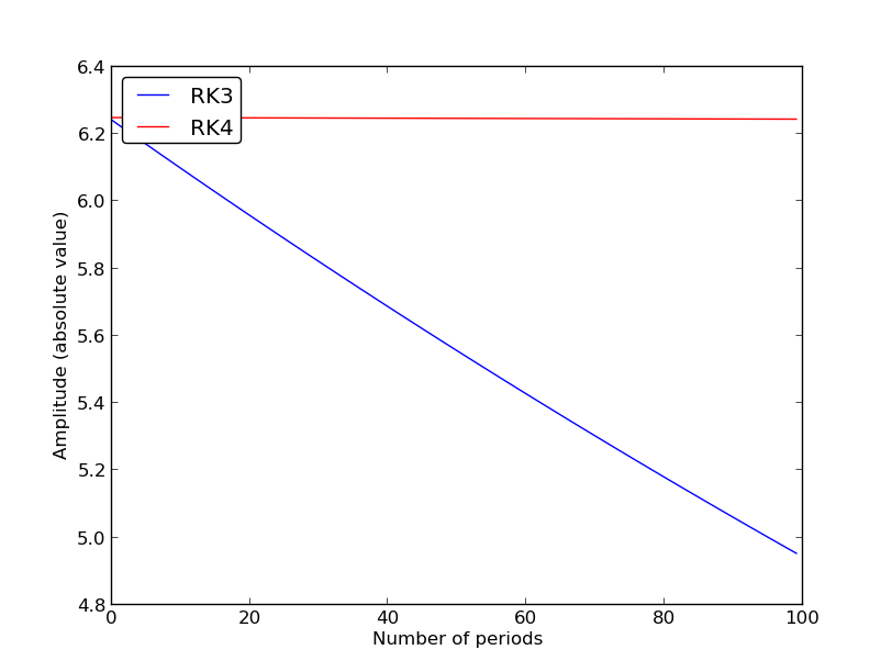
The amplitude as it changes over 100 periods for RK3 and RK4
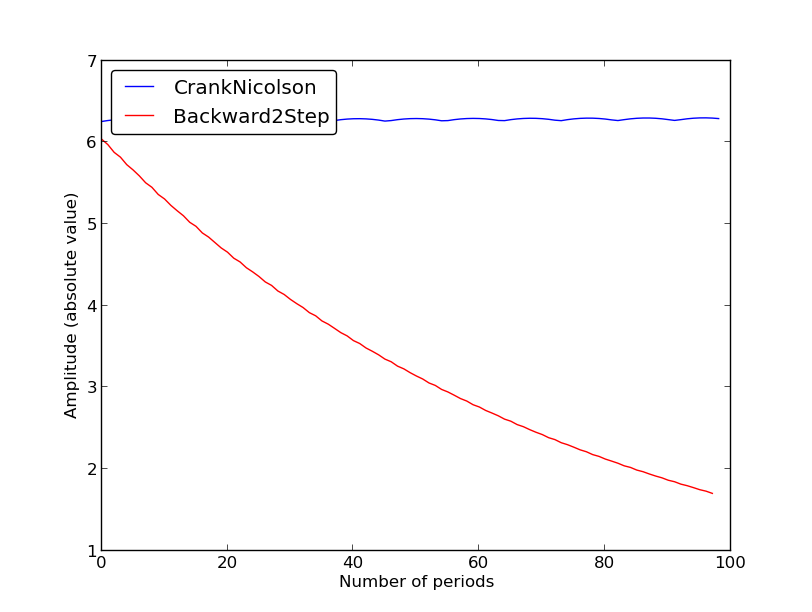
The amplitude as it changes over 100 periods for Crank-Nicolson and Backward 2 step
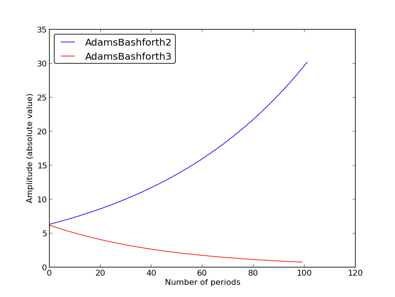
The amplitude as it changes over 100 periods for Adams-Bashforth 2 and 3
Filename: vib_amplitude_errors.
Problem 1.14: Minimize memory usage of a simple vibration solver
We consider the model problem \(u''+\omega^2 u = 0\), \(u(0)=I\), \(u'(0)=V\),
solved by a second-order finite difference scheme. A standard implementation
typically employs an array u for storing all the \(u^n\) values. However,
at some time level n+1 where we want to compute u[n+1], all we need
of previous u values are from level n and n-1. We can therefore avoid
storing the entire array u, and instead work with u[n+1], u[n],
and u[n-1], named as u, u_n, u_nmp1, for instance. Another
possible naming convention is u, u_n[0], u_n[-1].
Store the solution in a file
for later visualization. Make a test function that verifies the implementation
by comparing with the another code for the same problem.
Filename: vib_memsave0.
Problem 1.15: Minimize memory usage of a general vibration solver
The program vib.py stores the complete
solution \(u^0,u^1,\ldots,u^{N_t}\) in memory, which is convenient for
later plotting. Make a memory minimizing version of this program
where only the last three \(u^{n+1}\), \(u^n\), and \(u^{n-1}\) values are
stored in memory under the names u, u_n, and u_nm1 (this is the
naming convention used in this book).
Write each computed \((t_{n+1}, u^{n+1})\) pair to
file. Visualize the data in the file (a cool solution is to read one
line at a time and plot the \(u\) value using the line-by-line plotter
in the visualize_front_ascii function - this technique makes it
trivial to visualize very long time simulations).
Filename: vib_memsave.
Exercise 1.16: Implement the Euler-Cromer scheme for the generalized model
We consider the generalized model problem
a) Implement the Euler-Cromer method from the section The Euler-Cromer scheme for the generalized model.
b) We expect the Euler-Cromer method to have first-order convergence rate. Make a unit test based on this expectation.
c) Consider a system with \(m=4\), \(f(v)=b|v|v\), \(b=0.2\), \(s=2u\), \(F=0\). Compute the solution using the centered difference scheme from the section A centered scheme for linear damping and the Euler-Cromer scheme for the longest possible time step \(\Delta t\). We can use the result from the case without damping, i.e., the largest \(\Delta t= 2/\omega\), \(\omega\approx \sqrt{0.5}\) in this case, but since \(b\) will modify the frequency, we take the longest possible time step as a safety factor 0.9 times \(2/\omega\). Refine \(\Delta t\) three times by a factor of two and compare the two curves.
Filename: vib_EulerCromer.
Problem 1.17: Interpret \([D_tD_t u]^n\) as a forward-backward difference
Show that the difference \([D_t D_tu]^n\) is equal to \([D_t^+D_t^-u]^n\) and \(D_t^-D_t^+u]^n\). That is, instead of applying a centered difference twice one can alternatively apply a mixture of forward and backward differences.
Filename: vib_DtDt_fw_bw.
Exercise 1.18: Analysis of the Euler-Cromer scheme
The Euler-Cromer scheme for the model problem \(u^{\prime\prime} + \omega^2 u =0\), \(u(0)=I\), \(u^{\prime}(0)=0\), is given in (55)-(54). Find the exact discrete solutions of this scheme and show that the solution for \(u^n\) coincides with that found in the section Analysis of the numerical scheme.
Hint. Use an “ansatz” \(u^n=I\exp{(i\tilde\omega\Delta t\,n)}\) and \(v^n=qu^n\), where \(\tilde\omega\) and \(q\) are unknown parameters. The following formula is handy:
