Applications of vibration models
The following text derives some of the most well-known physical problems that lead to second-order ODE models of the type addressed in this book. We consider a simple spring-mass system; thereafter extended with nonlinear spring, damping, and external excitation; a spring-mass system with sliding friction; a simple and a physical (classical) pendulum; and an elastic pendulum.
Oscillating mass attached to a spring
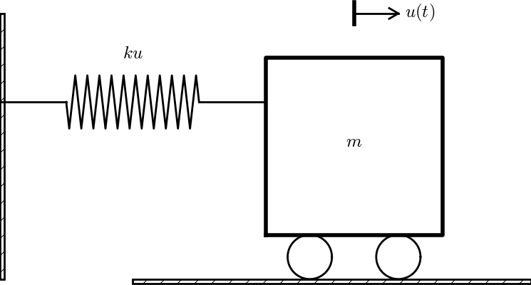
Simple oscillating mass
The most fundamental mechanical vibration system is depicted in Figure Simple oscillating mass. A body with mass \(m\) is attached to a spring and can move horizontally without friction (in the wheels). The position of the body is given by the vector \(\boldsymbol{r}(t) = u(t)\boldsymbol{i}\), where \(\boldsymbol{i}\) is a unit vector in \(x\) direction. There is only one force acting on the body: a spring force \(\boldsymbol{F}_s =-ku\boldsymbol{i}\), where \(k\) is a constant. The point \(x=0\), where \(u=0\), must therefore correspond to the body’s position where the spring is neither extended nor compressed, so the force vanishes.
The basic physical principle that governs the motion of the body is Newton’s second law of motion: \(\boldsymbol{F}=m\boldsymbol{a}\), where \(\boldsymbol{F}\) is the sum of forces on the body, \(m\) is its mass, and \(\boldsymbol{a}=\ddot\boldsymbol{r}\) is the acceleration. We use the dot for differentiation with respect to time, which is usual in mechanics. Newton’s second law simplifies here to \(-\boldsymbol{F}_s=m\ddot u\boldsymbol{i}\), which translates to
Two initial conditions are needed: \(u(0)=I\), \(\dot u(0)=V\). The ODE problem is normally written as
It is not uncommon to divide by \(m\) and introduce the frequency \(\omega = \sqrt{k/m}\):
This is the model problem in the first part of this chapter, with the small difference that we write the time derivative of \(u\) with a dot above, while we used \(u^{\prime}\) and \(u^{\prime\prime}\) in previous parts of the book.
Since only one scalar mathematical quantity, \(u(t)\), describes the complete motion, we say that the mechanical system has one degree of freedom (DOF).
Scaling
For numerical simulations it is very convenient to scale (120) and thereby get rid of the problem of finding relevant values for all the parameters \(m\), \(k\), \(I\), and \(V\). Since the amplitude of the oscillations are dictated by \(I\) and \(V\) (or more precisely, \(V/\omega\)), we scale \(u\) by \(I\) (or \(V/\omega\) if \(I=0\)):
The time scale \(t_c\) is normally chosen as the inverse period \(2\pi/\omega\) or angular frequency \(1/\omega\), most often as \(t_c=1/\omega\). Inserting the dimensionless quantities \(\bar u\) and \(\bar t\) in (120) results in the scaled problem
where \(\beta\) is a dimensionless number. Any motion that starts from rest (\(V=0\)) is free of parameters in the scaled model!
The physics
The typical physics of the system in Figure Simple oscillating mass can be described as follows. Initially, we displace the body to some position \(I\), say at rest (\(V=0\)). After releasing the body, the spring, which is extended, will act with a force \(-kI\boldsymbol{i}\) and pull the body to the left. This force causes an acceleration and therefore increases velocity. The body passes the point \(x=0\), where \(u=0\), and the spring will then be compressed and act with a force \(kx\boldsymbol{i}\) against the motion and cause retardation. At some point, the motion stops and the velocity is zero, before the spring force \(kx\boldsymbol{i}\) has worked long enough to push the body in positive direction. The result is that the body accelerates back and forth. As long as there is no friction forces to damp the motion, the oscillations will continue forever.
General mechanical vibrating system
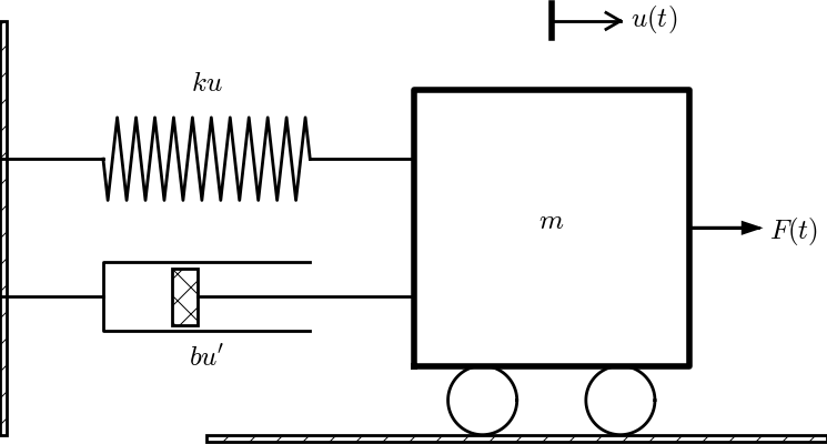
General oscillating system
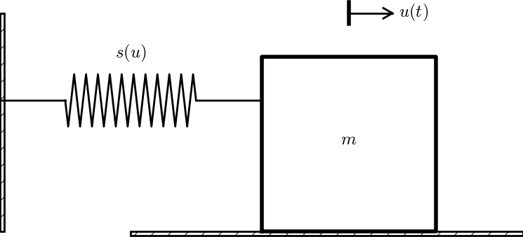
The mechanical system in Figure Simple oscillating mass can easily be extended to the more general system in Figure General oscillating system, where the body is attached to a spring and a dashpot, and also subject to an environmental force \(F(t)\boldsymbol{i}\). The system has still only one degree of freedom since the body can only move back and forth parallel to the \(x\) axis. The spring force was linear, \(\boldsymbol{F}_s=-ku\boldsymbol{i}\), in the section Oscillating mass attached to a spring, but in more general cases it can depend nonlinearly on the position. We therefore set \(\boldsymbol{F}_s=s(u)\boldsymbol{i}\). The dashpot, which acts as a damper, results in a force \(\boldsymbol{F}_d\) that depends on the body’s velocity \(\dot u\) and that always acts against the motion. The mathematical model of the force is written \(\boldsymbol{F}_d =f(\dot u)\boldsymbol{i}\). A positive \(\dot u\) must result in a force acting in the positive \(x\) direction. Finally, we have the external environmental force \(\boldsymbol{F}_e = F(t)\boldsymbol{i}\).
Newton’s second law of motion now involves three forces:
The common mathematical form of the ODE problem is
This is the generalized problem treated in the last part of the present chapter, but with prime denoting the derivative instead of the dot.
The most common models for the spring and dashpot are linear: \(f(\dot u) =b\dot u\) with a constant \(b\geq 0\), and \(s(u)=ku\) for a constant \(k\).
Scaling
A specific scaling requires specific choices of \(f\), \(s\), and \(F\). Suppose we have
We introduce dimensionless variables as usual, \(\bar u = u/u_c\) and \(\bar t = t/t_c\). The scale \(u_c\) depends both on the initial conditions and \(F\), but as time grows, the effect of the initial conditions die out and \(F\) will drive the motion. Inserting \(\bar u\) and \(\bar t\) in the ODE gives
We divide by \(u_c/t_c^2\) and demand the coefficients of the \(\bar u\) and the forcing term from \(F(t)\) to have unit coefficients. This leads to the scales
The scaled ODE becomes
where there are two dimensionless numbers:
The \(\beta\) number measures the size of the damping term (relative to unity) and is assumed to be small, basically because \(b\) is small. The \(\phi\) number is the ratio of the time scale of free vibrations and the time scale of the forcing. The scaled initial conditions have two other dimensionless numbers as values:
A sliding mass attached to a spring
Consider a variant of the oscillating body in the section Oscillating mass attached to a spring and Figure Simple oscillating mass: the body rests on a flat surface, and there is sliding friction between the body and the surface. Figure Sketch of a body sliding on a surface depicts the problem.
Sketch of a body sliding on a surface
The body is attached to a spring with spring force \(-s(u)\boldsymbol{i}\). The friction force is proportional to the normal force on the surface, \(-mg\boldsymbol{j}\), and given by \(-f(\dot u)\boldsymbol{i}\), where
Here, \(\mu\) is a friction coefficient. With the signum function
we can simply write \(f(\dot u) = \mu mg\,\hbox{sign}(\dot u)\)
(the sign function is implemented by numpy.sign).
The equation of motion becomes
A jumping washing machine
A washing machine is placed on four springs with efficient dampers. If the machine contains just a few clothes, the circular motion of the machine induces a sinusoidal external force and the machine will jump up and down if the frequency of the external force is close to the natural frequency of the machine and its spring-damper system.
Motion of a pendulum
Simple pendulum
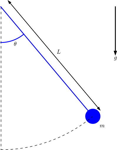
A classical problem in mechanics is the motion of a pendulum. We first consider a simple pendulum (sometimes also called a mathematical pendulum): a small body of mass \(m\) is attached to a massless wire and can oscillate back and forth in the gravity field. Figure Sketch of a simple pendulum shows a sketch of the problem.
Sketch of a simple pendulum
The motion is governed by Newton’s 2nd law, so we need to find expressions for the forces and the acceleration. Three forces on the body are considered: an unknown force \(S\) from the wire, the gravity force \(mg\), and an air resistance force, \(\frac{1}{2}C_D\varrho A|v|v\), hereafter called the drag force, directed against the velocity of the body. Here, \(C_D\) is a drag coefficient, \(\varrho\) is the density of air, \(A\) is the cross section area of the body, and \(v\) is the magnitude of the velocity.
We introduce a coordinate system with polar coordinates and unit vectors \({\boldsymbol{i}_r}\) and \(\boldsymbol{i}_{\theta}\) as shown in Figure Forces acting on a simple pendulum. The position of the center of mass of the body is
where \(\boldsymbol{i}\) and \(\boldsymbol{j}\) are unit vectors in the corresponding Cartesian coordinate system in the \(x\) and \(y\) directions, respectively. We have that \({\boldsymbol{i}_r} = \cos\theta\boldsymbol{i} +\sin\theta\boldsymbol{j}\).
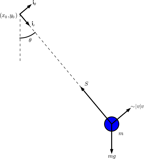
Forces acting on a simple pendulum
The forces are now expressed as follows.
- Wire force: \(-S{\boldsymbol{i}_r}\)
- Gravity force: \(-mg\boldsymbol{j} = mg(-\sin\theta\,\boldsymbol{i}_{\theta} + \cos\theta\,{\boldsymbol{i}_r})\)
- Drag force: \(-\frac{1}{2}C_D\varrho A |v|v\,\boldsymbol{i}_{\theta}\)
Since a positive velocity means movement in the direction of \(\boldsymbol{i}_{\theta}\), the drag force must be directed along \(-\boldsymbol{i}_{\theta}\) so it works against the motion. We assume motion in air so that the added mass effect can be neglected (for a spherical body, the added mass is \(\frac{1}{2}\varrho V\), where \(V\) is the volume of the body). Also the buoyancy effect can be neglected for motion in the air when the density difference between the fluid and the body is so significant.
The velocity of the body is found from \(\boldsymbol{r}\):
since \(\frac{d}{d\theta}{\boldsymbol{i}_r} = \boldsymbol{i}_{\theta}\). It follows that \(v=|\boldsymbol{v}|=L\dot\theta\). The acceleration is
since \(\frac{d}{d\theta}\boldsymbol{i}_{\theta} = -{\boldsymbol{i}_r}\).
Newton’s 2nd law of motion becomes
leading to two component equations
From (124) we get an expression for \(S=mg\cos\theta + L\dot\theta^2\), and from (125) we get a differential equation for the angle \(\theta(t)\). This latter equation is ordered as
Two initial conditions are needed: \(\theta=\Theta\) and \(\dot\theta = \Omega\). Normally, the pendulum motion is started from rest, which means \(\Omega =0\).
Equation (126) fits the general model used in (71) in the section Generalization: damping, nonlinearities, and excitation if we define \(u=\theta\), \(f(u^{\prime}) = \frac{1}{2}C_D\varrho AL|\dot u|\dot u\), \(s(u) = L^{-1}mg\sin u\), and \(F=0\). If the body is a sphere with radius \(R\), we can take \(C_D=0.4\) and \(A=\pi R^2\). Exercise 1.25: Simulate a simple pendulum asks you to scale the equations and carry out specific simulations with this model.
Physical pendulum
The motion of a compound or physical pendulum where the wire is a rod with mass, can be modeled very similarly. The governing equation is \(I\boldsymbol{a} = \boldsymbol{T}\) where \(I\) is the moment of inertia of the entire body about the point \((x_0,y_0)\), and \(\boldsymbol{T}\) is the sum of moments of the forces with respect to \((x_0,y_0)\). The vector equation reads
The component equation in \(\boldsymbol{i}_{\theta}\) direction gives the equation of motion for \(\theta(t)\):
Dynamic free body diagram during pendulum motion
Usually one plots the mathematical quantities as functions of time to visualize the solution of ODE models. Exercise 1.25: Simulate a simple pendulum asks you to do this for the motion of a pendulum in the previous section. However, sometimes it is more instructive to look at other types of visualizations. For example, we have the pendulum and the free body diagram in Figures Sketch of a simple pendulum and Forces acting on a simple pendulum. We may think of these figures as animations in time instead. Especially the free body diagram will show both the motion of the pendulum and the size of the forces during the motion. The present section exemplifies how to make such a dynamic body diagram.
The drag force is magnified 5 times!
Dynamic physical sketches, coupled to the numerical solution of differential equations, requires a program to produce a sketch for the situation at each time level. Pysketcher is such a tool. In fact (and not surprising!) Figures Sketch of a simple pendulum and Forces acting on a simple pendulum were drawn using Pysketcher. The details of the drawings are explained in the Pysketcher tutorial. Here, we outline how this type of sketch can be used to create an animated free body diagram during the motion of a pendulum.
Pysketcher is actually a layer of useful abstractions on top of standard plotting packages. This means that we in fact apply Matplotlib to make the animated free body diagram, but instead of dealing with a wealth of detailed Matplotlib commands, we can express the drawing in terms of more high-level objects, e.g., objects for the wire, angle \(\theta\), body with mass \(m\), arrows for forces, etc. When the position of these objects are given through variables, we can just couple those variables to the dynamic solution of our ODE and thereby make a unique drawing for each \(\theta\) value in a simulation.
Writing the solver
Let us start with the most familiar part of the current problem: writing the solver function. We use Odespy for this purpose. We also work with dimensionless equations. Since \(\theta\) can be viewed as dimensionless, we only need to introduce a dimensionless time, here taken as \(\bar t = t/\sqrt{L/g}\). The resulting dimensionless mathematical model for \(\theta\), the dimensionless angular velocity \(\omega\), the dimensionless wire force \(\bar S\), and the dimensionless drag force \(\bar D\) is then
with
as a dimensionless parameter expressing the ratio of the drag force and the gravity force. The dimensionless \(\omega\) is made non-dimensional by the time, so \(\omega\sqrt{L/g}\) is the corresponding angular frequency with dimensions.
A suitable function for computing (128)-(131) is listed below.
def simulate(alpha, Theta, dt, T):
    import odespy

    def f(u, t, alpha):
        omega, theta = u
        return [-alpha*omega*abs(omega) - sin(theta),
                omega]

    import numpy as np
    Nt = int(round(T/float(dt)))
    t = np.linspace(0, Nt*dt, Nt+1)
    solver = odespy.RK4(f, f_args=[alpha])
    solver.set_initial_condition([0, Theta])
    u, t = solver.solve(
        t, terminate=lambda u, t, n: abs(u[n,1]) < 1E-3)
    omega = u[:,0]
    theta = u[:,1]
    S = omega**2 + np.cos(theta)
    drag = -alpha*np.abs(omega)*omega
    return t, theta, omega, S, drag
Drawing the free body diagram
The sketch function below applies Pysketcher objects to build
a diagram like that in Figure Forces acting on a simple pendulum,
except that we have removed the rotation point \((x_0,y_0)\) and
the unit vectors in polar coordinates as these objects are not
important for an animated free body diagram.
import sys
try:
    from pysketcher import *
except ImportError:
    print 'Pysketcher must be installed from'
    print 'https://github.com/hplgit/pysketcher'
    sys.exit(1)

# Overall dimensions of sketch
H = 15.
W = 17.

drawing_tool.set_coordinate_system(
    xmin=0, xmax=W, ymin=0, ymax=H,
    axis=False)

def sketch(theta, S, mg, drag, t, time_level):
    """
    Draw pendulum sketch with body forces at a time level
    corresponding to time t. The drag force is in
    drag[time_level], the force in the wire is S[time_level],
    the angle is theta[time_level].
    """
    import math
    a = math.degrees(theta[time_level])  # angle in degrees
    L = 0.4*H         # Length of pendulum
    P = (W/2, 0.8*H)  # Fixed rotation point

    mass_pt = path.geometric_features()['end']
    rod = Line(P, mass_pt)

    mass = Circle(center=mass_pt, radius=L/20.)
    mass.set_filled_curves(color='blue')
    rod_vec = rod.geometric_features()['end'] - \
              rod.geometric_features()['start']
    unit_rod_vec = unit_vec(rod_vec)
    mass_symbol = Text('$m$', mass_pt + L/10*unit_rod_vec)

    rod_start = rod.geometric_features()['start']  # Point P
    vertical = Line(rod_start, rod_start + point(0,-L/3))

    def set_dashed_thin_blackline(*objects):
        """Set linestyle of objects to dashed, black, width=1."""
        for obj in objects:
            obj.set_linestyle('dashed')
            obj.set_linecolor('black')
            obj.set_linewidth(1)

    set_dashed_thin_blackline(vertical)
    set_dashed_thin_blackline(rod)
    angle = Arc_wText(r'$\theta$', rod_start, L/6, -90, a,
                      text_spacing=1/30.)

    magnitude = 1.2*L/2   # length of a unit force in figure
    force = mg[time_level]  # constant (scaled eq: about 1)
    force *= magnitude
    mg_force  = Force(mass_pt, mass_pt + force*point(0,-1),
                      '', text_pos='end')
    force = S[time_level]
    force *= magnitude
    rod_force = Force(mass_pt, mass_pt - force*unit_vec(rod_vec),
                      '', text_pos='end',
                      text_spacing=(0.03, 0.01))
    force = drag[time_level]
    force *= magnitude
    air_force = Force(mass_pt, mass_pt -
                      force*unit_vec((rod_vec[1], -rod_vec[0])),
                      '', text_pos='end',
                      text_spacing=(0.04,0.005))

    body_diagram = Composition(
        {'mg': mg_force, 'S': rod_force, 'air': air_force,
         'rod': rod, 'body': mass
         'vertical': vertical, 'theta': angle,})

    body_diagram.draw(verbose=0)
    drawing_tool.savefig('tmp_%04d.png' % time_level, crop=False)
    # (No cropping: otherwise movies will be very strange!)
Making the animated free body diagram
It now remains to couple the simulate and sketch functions.
We first run simulate:
from math import pi, radians, degrees
import numpy as np
alpha = 0.4
period = 2*pi   # Use small theta approximation
T = 12*period   # Simulate for 12 periods
dt = period/40  # 40 time steps per period
a = 70          # Initial amplitude in degrees
Theta = radians(a)

t, theta, omega, S, drag = simulate(alpha, Theta, dt, T)
The next step is to run through the time levels in the simulation and make a sketch at each level:
for time_level, t_ in enumerate(t):
    sketch(theta, S, mg, drag, t_, time_level)
The individual sketches are (by the sketch function) saved in files
with names tmp_%04d.png. These can be combined to videos using
(e.g.) ffmpeg. A complete function animate for running the
simulation and creating video files is
listed below.
def animate():
    # Clean up old plot files
    import os, glob
    for filename in glob.glob('tmp_*.png') + glob.glob('movie.*'):
        os.remove(filename)
    # Solve problem
    from math import pi, radians, degrees
    import numpy as np
    alpha = 0.4
    period = 2*pi   # Use small theta approximation
    T = 12*period   # Simulate for 12 periods
    dt = period/40  # 40 time steps per period
    a = 70          # Initial amplitude in degrees
    Theta = radians(a)

    t, theta, omega, S, drag = simulate(alpha, Theta, dt, T)

    # Visualize drag force 5 times as large
    drag *= 5
    mg = np.ones(S.size)  # Gravity force (needed in sketch)

    # Draw animation
    import time
    for time_level, t_ in enumerate(t):
        sketch(theta, S, mg, drag, t_, time_level)
        time.sleep(0.2)  # Pause between each frame on the screen

    # Make videos
    prog = 'ffmpeg'
    filename = 'tmp_%04d.png'
    fps = 6
    codecs = {'flv': 'flv', 'mp4': 'libx264',
              'webm': 'libvpx', 'ogg': 'libtheora'}
    for ext in codecs:
        lib = codecs[ext]
        cmd = '%(prog)s -i %(filename)s -r %(fps)s ' % vars()
        cmd += '-vcodec %(lib)s movie.%(ext)s' % vars()
        print(cmd)
        os.system(cmd)
Motion of an elastic pendulum
Consider a pendulum as in Figure Sketch of a simple pendulum, but this time the wire is elastic. The length of the wire when it is not stretched is \(L_0\), while \(L(t)\) is the stretched length at time \(t\) during the motion.
Stretching the elastic wire a distance \(\Delta L\) gives rise to a spring force \(k\Delta L\) in the opposite direction of the stretching. Let \(\boldsymbol{n}\) be a unit normal vector along the wire from the point \(\boldsymbol{r}_0=(x_0,y_0)\) and in the direction of \(\boldsymbol{i}_{\theta}\), see Figure Forces acting on a simple pendulum for definition of \((x_0,y_0)\) and \(\boldsymbol{i}_{\theta}\). Obviously, we have \(\boldsymbol{n}=\boldsymbol{i}_{\theta}\), but in this modeling of an elastic pendulum we do not need polar coordinates. Instead, it is more straightforward to develop the equation in Cartesian coordinates.
A mathematical expression for \(\boldsymbol{n}\) is
where \(L(t)=||\boldsymbol{r}-\boldsymbol{r}_0||\) is the current length of the elastic wire. The position vector \(\boldsymbol{r}\) in Cartesian coordinates reads \(\boldsymbol{r}(t) = x(t)\boldsymbol{i} + y(t)\boldsymbol{j}\), where \(\boldsymbol{i}\) and \(\boldsymbol{j}\) are unit vectors in the \(x\) and \(y\) directions, respectively. It is convenient to introduce the Cartesian components \(n_x\) and \(n_y\) of the normal vector:
The stretch \(\Delta L\) in the wire is
The force in the wire is then \(-S\boldsymbol{n}=-k\Delta L\boldsymbol{n}\).
The other forces are the gravity and the air resistance, just as in Figure Forces acting on a simple pendulum. For motion in air we can neglect the added mass and buoyancy effects. The main difference is that we have a model for \(S\) in terms of the motion (as soon as we have expressed \(\Delta L\) by \(\boldsymbol{r}\)). For simplicity, we drop the air resistance term (but Exercise 1.27: Simulate an elastic pendulum with air resistance asks you to include it).
Newton’s second law of motion applied to the body now results in
The two components of (132) are
Remarks about an elastic vs a non-elastic pendulum
Note that the derivation of the ODEs for an elastic pendulum is more straightforward than for a classical, non-elastic pendulum, since we avoid the details with polar coordinates, but instead work with Newton’s second law directly in Cartesian coordinates. The reason why we can do this is that the elastic pendulum undergoes a general two-dimensional motion where all the forces are known or expressed as functions of \(x(t)\) and \(y(t)\), such that we get two ordinary differential equations. The motion of the non-elastic pendulum, on the other hand, is constrained: the body has to move along a circular path, and the force \(S\) in the wire is unknown.
The non-elastic pendulum therefore leads to a differential-algebraic equation, i.e., ODEs for \(x(t)\) and \(y(t)\) combined with an extra constraint \((x-x_0)^2 + (y-y_0)^2 = L^2\) ensuring that the motion takes place along a circular path. The extra constraint (equation) is compensated by an extra unknown force \(-S\boldsymbol{n}\). Differential-algebraic equations are normally hard to solve, especially with pen and paper. Fortunately, for the non-elastic pendulum we can do a trick: in polar coordinates the unknown force \(S\) appears only in the radial component of Newton’s second law, while the unknown degree of freedom for describing the motion, the angle \(\theta(t)\), is completely governed by the asimuthal component. This allows us to decouple the unknowns \(S\) and \(\theta\). But this is a kind of trick and not a widely applicable method. With an elastic pendulum we use straightforward reasoning with Newton’s 2nd law and arrive at a standard ODE problem that (after scaling) is easy solve on a computer.
Initial conditions
What is the initial position of the body? We imagine that first the pendulum hangs in equilibrium in its vertical position, and then it is displaced an angle \(\Theta\). The equilibrium position is governed by the ODEs with the accelerations set to zero. The \(x\) component leads to \(x(t)=x_0\), while the \(y\) component gives
since \(n_y=-11\) in this position. The corresponding \(y\) value is then from \(n_y=-1\):
Let us now choose \((x_0,y_0)\) such that the body is at the origin in the equilibrium position:
Displacing the body an angle \(\Theta\) to the right leads to the initial position
The initial velocities can be set to zero: \(x'(0)=y'(0)=0\).
The complete ODE problem
We can summarize all the equations as follows:
We insert \(n_x\) and \(n_y\) in the ODEs:
Scaling
The elastic pendulum model can be used to study both an elastic pendulum and a classic, non-elastic pendulum. The latter problem is obtained by letting \(k\rightarrow\infty\). Unfortunately, a serious problem with the ODEs (136)-(137) is that for large \(k\), we have a very large factor \(k/m\) multiplied by a very small number \(1-L_0/L\), since for large \(k\), \(L\approx L_0\) (very small deformations of the wire). The product is subject to significant round-off errors for many relevant physical values of the parameters. To circumvent the problem, we introduce a scaling. This will also remove physical parameters from the problem such that we end up with only one dimensionless parameter, closely related to the elasticity of the wire. Simulations can then be done by setting just this dimensionless parameter.
The characteristic length can be taken such that in equilibrium, the scaled length is unity, i.e., the characteristic length is \(L_0+mg/k\):
We must then also work with the scaled length \(\bar L = L/(L_0+mg/k)\).
Introducing \(\bar t=t/t_c\), where \(t_c\) is a characteristic time we have to decide upon later, one gets
For a non-elastic pendulum with small angles, we know that the frequency of the oscillations are \(\omega = \sqrt{L/g}\). It is therefore natural to choose a similar expression here, either the length in the equilibrium position,
or simply the unstretched length,
These quantities are not very different (since the elastic model is valid only for quite small elongations), so we take the latter as it is the simplest one.
The ODEs become
We can now identify a dimensionless number
which is the ratio of the unstretched length and the stretched length in equilibrium. The non-elastic pendulum will have \(\beta =1\) (\(k\rightarrow\infty\)). With \(\beta\) the ODEs read
We have here added a parameter \(\epsilon\), which is an additional downward stretch of the wire at \(t=0\). This parameter makes it possible to do a desired test: vertical oscillations of the pendulum. Without \(\epsilon\), starting the motion from \((0,0)\) with zero velocity will result in \(x=y=0\) for all times (also a good test!), but with an initial stretch so the body’s position is \((0,\epsilon)\), we will have oscillatory vertical motion with amplitude \(\epsilon\) (see Exercise 1.26: Simulate an elastic pendulum).
Remark on the non-elastic limit
We immediately see that as \(k\rightarrow\infty\) (i.e., we obtain a non-elastic pendulum), \(\beta\rightarrow 1\), \(\bar L\rightarrow 1\), and we have very small values \(1-\beta\bar L^{-1}\) divided by very small values \(1-\beta\) in the ODEs. However, it turns out that we can set \(\beta\) very close to one and obtain a path of the body that within the visual accuracy of a plot does not show any elastic oscillations. (Should the division of very small values become a problem, one can study the limit by L’Hospital’s rule:
and use the limit \(\bar L^{-1}\) in the ODEs for \(\beta\) values very close to 1.)
Vehicle on a bumpy road
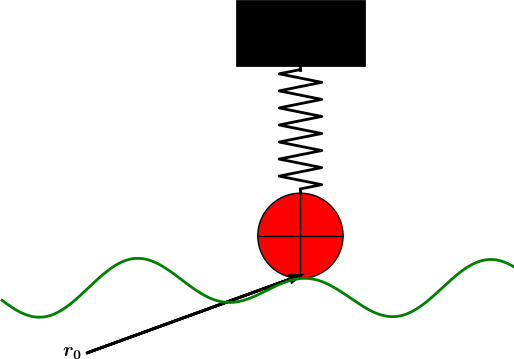
Sketch of one-wheel vehicle on a bumpy road
We consider a very simplistic vehicle, on one wheel, rolling along a bumpy road. The oscillatory nature of the road will induce an external forcing on the spring system in the vehicle and cause vibrations. Figure Sketch of one-wheel vehicle on a bumpy road outlines the situation.
To derive the equation that governs the motion, we must first establish the position vector of the black mass at the top of the spring. Suppose the spring has length \(L\) without any elongation or compression, suppose the radius of the wheel is \(R\), and suppose the height of the black mass at the top is \(H\). With the aid of the \(\boldsymbol{r}_0\) vector in Figure Sketch of one-wheel vehicle on a bumpy road, the position \(\boldsymbol{r}\) of the center point of the mass is
where \(u\) is the elongation or compression in the spring according to the (unknown and to be computed) vertical displacement \(u\) relative to the road. If the vehicle travels with constant horizontal velocity \(v\) and \(h(x)\) is the shape of the road, then the vector \(\boldsymbol{r}_0\) is
if the motion starts from \(x=0\) at time \(t=0\).
The forces on the mass is the gravity, the spring force, and an optional damping force that is proportional to the vertical velocity \(\dot u\). Newton’s second law of motion then tells that
This leads to
To simplify a little bit, we omit the gravity force \(mg\) in comparison with the other terms. Introducing \(u'\) for \(\dot u\) then gives a standard damped, vibration equation with external forcing:
Since the road is normally known just as a set of array values, \(h''\) must be computed by finite differences. Let \(\Delta x\) be the spacing between measured values \(h_i= h(i\Delta x)\) on the road. The discrete second-order derivative \(h''\) reads
We may for maximum simplicity set the end points as \(q_0=q_1\) and \(q_{N_x}=q_{N_x-1}\). The term \(-mh''(vt)v^2\) corresponds to a force with discrete time values
This force can be directly used in a numerical model
Software for computing \(u\) and also making an animated sketch of the motion like we did in the section Dynamic free body diagram during pendulum motion is found in a separate project on the web: https://github.com/hplgit/bumpy. You may start looking at the tutorial.
Bouncing ball
A bouncing ball is a ball in free vertically fall until it impacts the ground, but during the impact, some kinetic energy is lost, and a new motion upwards with reduced velocity starts. After the motion is retarded, a new free fall starts, and the process is repeated. At some point the velocity close to the ground is so small that the ball is considered to be finally at rest.
The motion of the ball falling in air is governed by Newton’s second law \(F=ma\), where \(a\) is the acceleration of the body, \(m\) is the mass, and \(F\) is the sum of all forces. Here, we neglect the air resistance so that gravity \(-mg\) is the only force. The height of the ball is denoted by \(h\) and \(v\) is the velocity. The relations between \(h\), \(v\), and \(a\),
combined with Newton’s second law gives the ODE model
or expressed alternatively as a system of first-order equations:
These equations govern the motion as long as the ball is away from the ground by a small distance \(\epsilon_h > 0\). When \(h<\epsilon_h\), we have two cases.
- The ball impacts the ground, recognized by a sufficiently large negative velocity (\(v<-\epsilon_v\)). The velocity then changes sign and is reduced by a factor \(C_R\), known as the coefficient of restitution. For plotting purposes, one may set \(h=0\).
- The motion stops, recognized by a sufficiently small velocity (\(|v|<\epsilon_v\)) close to the ground.
Two-body gravitational problem
Consider two astronomical objects \(A\) and \(B\) that attract each other by gravitational forces. \(A\) and \(B\) could be two stars in a binary system, a planet orbiting a star, or a moon orbiting a planet. Each object is acted upon by the gravitational force due to the other object. Consider motion in a plane (for simplicity) and let \((x_A,y_A)\) and \((x_B,y_B)\) be the positions of object \(A\) and \(B\), respectively.
The governing equations
Newton’s second law of motion applied to each object is all we need to set up a mathematical model for this physical problem:
where \(F\) is the gravitational force
where
and \(G\) is the gravitational constant: \(G=6.674\cdot 10^{-11}\hbox{ Nm}^2/\hbox{kg}^2\).
Scaling
A problem with these equations is that the parameters are very large (\(m_A\), \(m_B\), \(||\boldsymbol{r}||\)) or very small (\(G\)). The rotation time for binary stars can be very small and large as well. It is therefore advantageous to scale the equations. A natural length scale could be the initial distance between the objects: \(L=\boldsymbol{r}(0)\). We write the dimensionless quantities as
The gravity force is transformed to
so the first ODE for \(\boldsymbol{x}_A\) becomes
Assuming that quantities with a bar and their derivatives are around unity in size, it is natural to choose \(t_c\) such that the fraction \(Gm_Bt_c/L^2=1\):
From the other equation for \(\boldsymbol{x}_B\) we get another candidate for \(t_c\) with \(m_A\) instead of \(m_B\). Which mass we choose play a role if \(m_A\ll m_B\) or \(m_B\ll m_A\). One solution is to use the sum of the masses:
Taking a look at Kepler’s laws of planetary motion, the orbital period for a planet around the star is given by the \(t_c\) above, except for a missing factor of \(2\pi\), but that means that \(t_c^{-1}\) is just the angular frequency of the motion. Our characteristic time \(t_c\) is therefore highly relevant. Introducing the dimensionless number
we can write the dimensionless ODE as
In the limit \(m_A\ll m_B\), i.e., \(\alpha\ll 1\), object B stands still, say \(\bar\boldsymbol{x}_B=0\), and object A orbits according to
Solution in a special case: planet orbiting a star
To better see the motion, and that our scaling is reasonable, we introduce polar coordinates \(r\) and \(\theta\):
which means \(\bar\boldsymbol{x}_A\) can be written as \(\bar\boldsymbol{x}_A =r{\boldsymbol{i}_r}\). Since
we have
The equation of motion for mass A is then
The special case of circular motion, \(r=1\), fulfills the equations, since the latter equation then gives \(\dot\theta =\hbox{const}\) and the former then gives \(\dot\theta = 1\), i.e., the motion is \(r(t)=1\), \(\theta(t)=t\), with unit angular frequency as expected and period \(2\pi\) as expected.
Electric circuits
Although the term “mechanical vibrations” is used in the present book, we must mention that the same type of equations arise when modeling electric circuits. The current \(I(t)\) in a circuit with an inductor with inductance \(L\), a capacitor with capacitance \(C\), and overall resistance \(R\), is governed by
where \(V(t)\) is the voltage source powering the circuit. This equation has the same form as the general model considered in the section Generalization: damping, nonlinearities, and excitation if we set \(u=I\), \(f(u^{\prime})=bu^{\prime}\) and define \(b=R/L\), \(s(u) = L^{-1}C^{-1}u\), and \(F(t)=\dot V(t)\).
Exercises
Exercise 1.22: Simulate resonance
We consider the scaled ODE model (122) from the section General mechanical vibrating system. After scaling, the amplitude of \(u\) will have a size about unity as time grows and the effect of the initial conditions die out due to damping. However, as \(\gamma\rightarrow 1\), the amplitude of \(u\) increases, especially if \(\beta\) is small. This effect is called resonance. The purpose of this exercise is to explore resonance.
a)
Figure out how the solver function in vib.py can be called
for the scaled ODE (122).
b) Run \(\gamma =5, 1.5, 1.1, 1\) for \(\beta=0.005, 0.05, 0.2\). For each \(\beta\) value, present an image with plots of \(u(t)\) for the four \(\gamma\) values.
Filename: resonance.
Exercise 1.23: Simulate oscillations of a sliding box
Consider a sliding box on a flat surface as modeled in the section A sliding mass attached to a spring. As spring force we choose the nonlinear formula
a) Plot \(g(u)=\alpha^{-1}\tanh(\alpha u)\) for various values of \(\alpha\). Assume \(u\in [-1,1]\).
b) Scale the equations using \(I\) as scale for \(u\) and \(\sqrt{m/k}\) as time scale.
c) Implement the scaled model in b). Run it for some values of the dimensionless parameters.
Filename: sliding_box.
Exercise 1.24: Simulate a bouncing ball
The section Bouncing ball presents a model for a bouncing ball. Choose one of the two ODE formulation, (152) or (153)-(154), and simulate the motion of a bouncing ball. Plot \(h(t)\). Think about how to plot \(v(t)\).
Hint. A naive implementation may get stuck in repeated impacts for large time step sizes. To avoid this situation, one can introduce a state variable that holds the mode of the motion: free fall, impact, or rest. Two consecutive impacts imply that the motion has stopped.
Filename: bouncing_ball.
Exercise 1.25: Simulate a simple pendulum
Simulation of simple pendulum can be carried out by using the mathematical model derived in the section Motion of a pendulum and calling up functionality in the vib.py file (i.e., solve the second-order ODE by centered finite differences).
a) Scale the model. Set up the dimensionless governing equation for \(\theta\) and expressions for dimensionless drag and wire forces.
b)
Write a function for computing
\(\theta\) and the dimensionless drag force and the force in the wire,
using the solver function in
the vib.py file. Plot these three quantities
below each other (in subplots) so the graphs can be compared.
Run two cases, first one in the limit of \(\Theta\) small and
no drag, and then a second one with \(\Theta=40\) degrees and \(\alpha=0.8\).
Filename: simple_pendulum.
Exercise 1.26: Simulate an elastic pendulum
The section Motion of an elastic pendulum describes a model for an elastic pendulum, resulting in a system of two ODEs. The purpose of this exercise is to implement the scaled model, test the software, and generalize the model.
a)
Write a function simulate
that can simulate an elastic pendulum using the scaled model.
The function should have the following arguments:
def simulate(
    beta=0.9,                 # dimensionless parameter
    Theta=30,                 # initial angle in degrees
    epsilon=0,                # initial stretch of wire
    num_periods=6,            # simulate for num_periods
    time_steps_per_period=60, # time step resolution
    plot=True,                # make plots or not
    ):
To set the total simulation time and the time step, we
use our knowledge of the scaled, classical, non-elastic pendulum:
\(u^{\prime\prime} + u = 0\), with solution
\(u = \Theta\cos \bar t\).
The period of these oscillations is \(P=2\pi\)
and the frequency is unity. The time
for simulation is taken as num_periods times \(P\). The time step
is set as \(P\) divided by time_steps_per_period.
The simulate function should return the arrays of
\(x\), \(y\), \(\theta\), and \(t\), where \(\theta = \tan^{-1}(x/(1-y))\) is
the angular displacement of the elastic pendulum corresponding to the
position \((x,y)\).
If plot is True, make a plot of \(\bar y(\bar t)\)
versus \(\bar x(\bar t)\), i.e., the physical motion
of the mass at \((\bar x,\bar y)\). Use the equal aspect ratio on the axis
such that we get a physically correct picture of the motion. Also
make a plot of \(\theta(\bar t)\), where \(\theta\) is measured in degrees.
If \(\Theta < 10\) degrees, add a plot that compares the solutions of
the scaled, classical, non-elastic pendulum and the elastic pendulum
(\(\theta(t)\)).
Although the mathematics here employs a bar over scaled quantities, the
code should feature plain names x for \(\bar x\), y for \(\bar y\), and
t for \(\bar t\) (rather than x_bar, etc.). These variable names make
the code easier to read and compare with the mathematics.
Hint 1.
Equal aspect ratio is set by plt.gca().set_aspect('equal') in
Matplotlib (import matplotlib.pyplot as plt)
and in SciTools by the command
plt.plot(..., daspect=[1,1,1], daspectmode='equal')
(provided you have done import scitools.std as plt).
Hint 2.
If you want to use Odespy to solve the equations, order the ODEs
like \(\dot \bar x, \bar x, \dot\bar y,\bar y\) such that
odespy.EulerCromer can be applied.
b) Write a test function for testing that \(\Theta=0\) and \(\epsilon=0\) gives \(x=y=0\) for all times.
c) Write another test function for checking that the pure vertical motion of the elastic pendulum is correct. Start with simplifying the ODEs for pure vertical motion and show that \(\bar y(\bar t)\) fulfills a vibration equation with frequency \(\sqrt{\beta/(1-\beta)}\). Set up the exact solution.
Write a test function that
uses this special case to verify the simulate function. There will
be numerical approximation errors present in the results from
simulate so you have to believe in correct results and set a
(low) tolerance that corresponds to the computed maximum error.
Use a small \(\Delta t\) to obtain a small numerical approximation error.
d)
Make a function demo(beta, Theta) for simulating an elastic pendulum with a
given \(\beta\) parameter and initial angle \(\Theta\). Use 600 time steps
per period to get every accurate results, and simulate for 3 periods.
Filename: elastic_pendulum.
Exercise 1.27: Simulate an elastic pendulum with air resistance
This is a continuation Exercise 1.26: Simulate an elastic pendulum.
Air resistance on the body with mass \(m\) can be modeled by the
force \(-\frac{1}{2}\varrho C_D A|\boldsymbol{v}|\boldsymbol{v}\),
where \(C_D\) is a drag coefficient (0.2 for a sphere), \(\varrho\)
is the density of air (1.2 \(\hbox{kg }\,{\hbox{m}}^{-3}\)), \(A\) is the
cross section area (\(A=\pi R^2\) for a sphere, where \(R\) is the radius),
and \(\boldsymbol{v}\) is the velocity of the body.
Include air resistance in the original model, scale the model,
write a function simulate_drag that is a copy of the simulate
function from Exercise 1.26: Simulate an elastic pendulum, but with the
new ODEs included, and show plots of how air resistance
influences the motion.
Filename: elastic_pendulum_drag.
Remarks
Test functions are challenging to construct for the problem with
air resistance. You can reuse the tests from
Exercise 1.27: Simulate an elastic pendulum with air resistance for simulate_drag,
but these tests does not verify the new terms arising from air
resistance.
Exercise 1.28: Implement the PEFRL algorithm
We consider the motion of a planet around a star (the section Two-body gravitational problem). The simplified case where one mass is very much bigger than the other and one object is at rest, results in the scaled ODE model
a) It is easy to show that \(x(t)\) and \(y(t)\) go like sine and cosine functions. Use this idea to derive the exact solution.
b) One believes that a planet may orbit a star for billions of years. We are now interested in how accurate methods we actually need for such calculations. A first task is to determine what the time interval of interest is in scaled units. Take the earth and sun as typical objects and find the characteristic time used in the scaling of the equations (\(t_c = \sqrt{L^3/(mG)}\)), where \(m\) is the mass of the sun, \(L\) is the distance between the sun and the earth, and \(G\) is the gravitational constant. Find the scaled time interval corresponding to one billion years.
c) Solve the equations using 4th-order Runge-Kutta and the Euler-Cromer methods. You may benefit from applying Odespy for this purpose. With each solver, simulate 10000 orbits and print the maximum position error and CPU time as a function of time step. Note that the maximum position error does not necessarily occur at the end of the simulation. The position error achieved with each solver will depend heavily on the size of the time step. Let the time step correspond to 200, 400, 800 and 1600 steps per orbit, respectively. Are the results as expected? Explain briefly. When you develop your program, have in mind that it will be extended with an implementation of the other algorithms (as requested in d) and e) later) and experiments with this algorithm as well.
d) Implement a solver based on the PEFRL method from the section The PEFRL 4th-order accurate algorithm. Verify its 4th-order convergence using an equation \(u'' + u = 0\).
e) The simulations done previously with the 4th-order Runge-Kutta and Euler-Cromer are now to be repeated with the PEFRL solver, so the code must be extended accordingly. Then run the simulations and comment on the performance of PEFRL compared to the other two.
f) Use the PEFRL solver to simulate 100000 orbits with a fixed time step corresponding to 1600 steps per period. Record the maximum error within each subsequent group of 1000 orbits. Plot these errors and fit (least squares) a mathematical function to the data. Print also the total CPU time spent for all 100000 orbits.
Now, predict the error and required CPU time for a simulation of 1 billion years (orbits). Is it feasible on today’s computers to simulate the planetary motion for one billion years?
Filename: vib_PEFRL.
Remarks
This exercise investigates whether it is feasible to predict planetary motion for the life time of a solar system.
