Scientific software engineering
Teaching material on scientific computing has traditionally been very focused on the mathematics and the applications, while details on how the computer is programmed to solve the problems have received little attention. Many end up writing as simple programs as possible, without being aware of much useful computer science technology that would increase the fun, efficiency, and reliability of the their scientific computing activities.
This chapter demonstrates a series of good practices and tools from modern computer science, using the simple mathematical problem \(u^{\prime}=-au\), \(u(0)=I\), such that we minimize the mathematical details and can go more in depth with implementations. The goal is to increase the technological quality of computer programming and make it match the more well-established quality of the mathematics of scientific computing.
The conventions and techniques outlined here will save you a lot of time when you incrementally extend software over time from simpler to more complicated problems. In particular, you will benefit from many good habits:
- new code is added in a modular fashion to a library (modules),
- programs are run through convenient user interfaces,
- it takes one quick command to let all your code undergo heavy testing,
- tedious manual work with running programs is automated,
- your scientific investigations are reproducible,
- scientific reports with top quality typesetting are produced both for paper and electronic devices.
Implementations with functions and modules
All previous examples in this book have implemented numerical algorithms as Python functions. This is a good style that readers are expected to adopt. However, this author has experienced that many students and engineers are inclined to make “flat” programs, i.e., a sequence of statements without any use of functions, just to get the problem solved as quickly as possible. Since this programming style is so widespread, especially among people with MATLAB experience, we shall look at the weaknesses of flat programs and show how they can be refactored into more reusable programs based on functions.
Mathematical problem and solution technique
We address the differential equation problem
where \(a\), \(I\), and \(T\) are prescribed parameters, and \(u(t)\) is the unknown function to be estimated. This mathematical model is relevant for physical phenomena featuring exponential decay in time, e.g., vertical pressure variation in the atmosphere, cooling of an object, and radioactive decay.
As we learned in the chapter The Forward Euler scheme, the time domain is discretized with points \(0 = t_0 < t_1 \cdots < t_{N_t}=T\), here with a constant spacing \(\Delta t\) between the mesh points: \(\Delta t = t_{n}-t_{n-1}\), \(n=1,\ldots,N_t\). Let \(u^n\) be the numerical approximation to the exact solution at \(t_n\). A family of popular numerical methods are provided by the \(\theta\) scheme,
for \(n=0,1,\ldots,N_t-1\). This formula produces the Forward Euler scheme when \(\theta=0\), the Backward Euler scheme when \(\theta=1\), and the Crank-Nicolson scheme when \(\theta=1/2\).
A first, quick implementation
Solving (197) in a program is very straightforward: just make a loop over \(n\) and evaluate the formula. The \(u(t_n\)) values for discrete \(n\) can be stored in an array. This makes it easy to also plot the solution. It would be natural to also add the exact solution curve \(u(t)=Ie^{-at}\) to the plot.
Many have programming habits that would lead them to write a simple program like this:
from numpy import *
from matplotlib.pyplot import *

A = 1
a = 2
T = 4
dt = 0.2
N = int(round(T/dt))
y = zeros(N+1)
t = linspace(0, T, N+1)
theta = 1
y[0] = A
for n in range(0, N):
    y[n+1] = (1 - (1-theta)*a*dt)/(1 + theta*dt*a)*y[n]

y_e = A*exp(-a*t) - y
error = y_e - y
E = sqrt(dt*sum(error**2))
print 'Norm of the error: %.3E' % E
plot(t, y, 'r--o')
t_e = linspace(0, T, 1001)
y_e = A*exp(-a*t_e)
plot(t_e, y_e, 'b-')
legend(['numerical, theta=%g' % theta, 'exact'])
xlabel('t')
ylabel('y')
show()
This program is easy to read, and as long as it is correct, many will claim that it has sufficient quality. Nevertheless, the program suffers from two serious flaws:
- The notation in the program does not correspond exactly to
the notation in the mathematical problem: the solution is called
yand corresponds to \(u\) in the mathematical description, the variableAcorresponds to the mathematical parameter \(I\),Nin the program is called \(N_t\) in the mathematics. - There are no comments in the program.
These kind of flaws quickly become crucial if present in code for complicated mathematical problems and code that is meant to be extended to other problems.
We also note that the program is flat in the sense that it does not contain functions. Usually, this is a bad habit, but let us first correct the two mentioned flaws.
A more decent program
A code of better quality arises from fixing the notation and adding comments:
from numpy import *
from matplotlib.pyplot import *

I = 1
a = 2
T = 4
dt = 0.2
Nt = int(round(T/dt))     # no of time intervals
u = zeros(Nt+1)           # array of u[n] values
t = linspace(0, T, Nt+1)  # time mesh
theta = 1                 # Backward Euler method

u[0] = I                  # assign initial condition
for n in range(0, Nt):    # n=0,1,...,Nt-1
    u[n+1] = (1 - (1-theta)*a*dt)/(1 + theta*dt*a)*u[n]

# Compute norm of the error
u_e = I*exp(-a*t) - u     # exact u at the mesh points
error = u_e - u
E = sqrt(dt*sum(error**2))
print 'Norm of the error: %.3E' % E

# Compare numerical (u) and exact solution (u_e) in a plot
plot(t, u, 'r--o')
t_e = linspace(0, T, 1001)       # very fine mesh for u_e
u_e = I*exp(-a*t_e)
plot(t_e, u_e, 'b-')
legend(['numerical, theta=%g' % theta, 'exact'])
xlabel('t')
ylabel('u')
show()
Comments in a program
There is obviously not just one way to comment a program, and opinions may differ as to what code should be commented. The guiding principle is, however, that comments should make the program easy to understand for the human eye. Do not comment obvious constructions, but focus on ideas and (“what happens in the next statements?”) and on explaining code that can be found complicated.
Refactoring into functions
At first sight, our updated program seems like a good starting point for playing around with the mathematical problem: we can just change parameters and rerun. Although such edit-and-rerun sessions are good for initial exploration, one will soon extend the experiments and start developing the code further. Say we want to compare \(\theta =0,1,0.5\) in the same plot. This extension requires changes all over the code and quickly leads to errors. To do something serious with this program, we have to break it into smaller pieces and make sure each piece is well tested, and ensure that the program is sufficiently general and can be reused in new contexts without changes. The next natural step is therefore to isolate the numerical computations and the visualization in separate Python functions. Such a rewrite of a code, without essentially changing the functionality, but just improve the quality of the code, is known as refactoring. After quickly putting together and testing a program, the next step is to refactor it so it becomes better prepared for extensions.
Program file vs IDE vs notebook
There are basically three different ways of working with Python code:
- One writes the code in a file, using a text editor (such as Emacs or Vim) and runs it in a terminal window.
- One applies an Integrated Development Environment (the simplest is IDLE, which comes with standard Python) containing a graphical user interface with an editor and an element where Python code can be run.
- One applies the Jupyter Notebook (previously known as IPython Notebook), which offers an interactive environment for Python code where plots are automatically inserted after the code, see Figure Experimental code in a notebook.
It appears that method 1 and 2 are quite equivalent, but the notebook encourages more experimental code and therefore also flat programs. Consequently, notebook users will normally need to think more about refactoring code and increase the use of functions after initial experimentation.
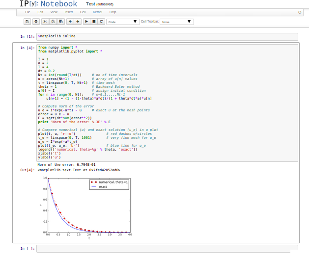
Experimental code in a notebook
Prefixing imported functions by the module name
Import statements of the form from module import * import
all functions and variables in module.py into the current file.
This is often referred to as “import star”, and
many find this convenient, but it is not considered as a good
programming style in Python.
For example, when doing
from numpy import *
from matplotlib.pyplot import *
we get mathematical functions like sin and exp as well as
MATLAB-style functions like linspace and plot, which can be called
by these well-known names. Unfortunately, it sometimes becomes
confusing to know where a particular function comes from, i.e., what
modules you need to import. Is a desired function from numpy or
matplotlib.pyplot? Or is it our own function? These questions are
easy to answer if functions in modules are prefixed by the module
name. Doing an additional from math import * is really crucial: now
sin, cos, and other mathematical functions are imported and their
names hide those previously imported from numpy. That is, sin is
now a sine function that accepts a float argument, not an array.
Doing the import such that module functions must have a prefix is generally recommended:
import numpy
import matplotlib.pyplot

t = numpy.linspace(0, T, Nt+1)
u_e = I*numpy.exp(-a*t)
matplotlib.pyplot.plot(t, u_e)
The modules numpy and matplotlib.pyplot are frequently used,
and since their full names are quite tedious to write,
two standard abbreviations
have evolved in the Python scientific computing community:
import numpy as np
import matplotlib.pyplot as plt

t = np.linspace(0, T, Nt+1)
u_e = I*np.exp(-a*t)
plt.plot(t, u_e)
The downside of prefixing functions by the module name is that mathematical expressions like \(e^{-at}\sin(2\pi t)\) get cluttered with module names,
numpy.exp(-a*t)*numpy.sin(2(numpy.pi*t)
# or
np.exp(-a*t)*np.sin(2*np.pi*t)
Such an expression looks like exp(-a*t)*sin(2*pi*t) in most other
programming languages. Similarly, np.linspace and plt.plot look
less familiar to people who are used to MATLAB and who have not
adopted Python’s prefix style. Whether to do from module import *
or import module depends on personal taste and the problem at
hand. In these writings we use from module import * in more basic,
shorter programs where similarity with MATLAB could be an
advantage. However, in reusable modules we prefix calls to module
functions by their function name, or do explicit import of the
needed functions:
from numpy import exp, sum, sqrt

def u_exact(t, I, a):
    return I*exp(-a*t)

error = u_exact(t, I, a) - u
E = sqrt(dt*sum(error**2))
Prefixing module functions or not
It can be advantageous to do a combination: mathematical functions
in formulas are imported without prefix, while module functions
in general are called with a prefix. For the numpy package we
can do
import numpy as np
from numpy import exp, sum, sqrt
such that mathematical expression can apply exp, sum, and sqrt
and hence look as close to the mathematical formulas as possible
(without a disturbing prefix).
Other calls to numpy function are done with the prefix, as in
np.linspace.
Implementing the numerical algorithm in a function
The solution formula (197) is completely general and
should be available as a Python function solver with all input data as
function arguments and all output data returned to the calling code.
With this solver function we can solve all types of problems
(195)-(196)
by an easy-to-read one-line statement:
u, t = solver(I=1, a=2, T=4, dt=0.2, theta=0.5)
Refactoring the numerical method in the previous flat program
in terms of a solver function and prefixing calls to
module functions by the module name leads to this code:
def solver(I, a, T, dt, theta):
    """Solve u'=-a*u, u(0)=I, for t in (0,T] with steps of dt."""
    dt = float(dt)               # avoid integer division
    Nt = int(round(T/dt))        # no of time intervals
    T = Nt*dt                    # adjust T to fit time step dt
    u = np.zeros(Nt+1)           # array of u[n] values
    t = np.linspace(0, T, Nt+1)  # time mesh

    u[0] = I                  # assign initial condition
    for n in range(0, Nt):    # n=0,1,...,Nt-1
        u[n+1] = (1 - (1-theta)*a*dt)/(1 + theta*dt*a)*u[n]
    return u, t
Tip: Always use a doc string to document a function
Python has a convention for documenting the purpose and usage of a function in a doc string: simply place the documentation in a one- or multi-line triple-quoted string right after the function header.
Be careful with unintended integer division
Note that we in the solver function explicitly covert dt to a
float object. If not, the updating formula for u[n+1] may evaluate
to zero because of integer division when theta, a, and dt are integers!
Do not have several versions of a code
One of the most serious flaws in computational work is to have several slightly different implementations of the same computational algorithms lying around in various program files. This is very likely to happen, because busy scientists often want to test a slight variation of a code to see what happens. A quick copy-and-edit does the task, but such quick hacks tend to survive. When a real correction is needed in the implementation, it is difficult to ensure that the correction is done in all relevant files. In fact, this is a general problem in programming, which has led to an important principle.
The DRY principle: Don’t repeat yourself
When implementing a particular functionality in a computer program, make sure this functionality and its variations are implemented in just one piece of code. That is, if you need to revise the implementation, there should be one and only one place to edit. It follows that you should never duplicate code (don’t repeat yourself!), and code snippets that are similar should be factored into one piece (function) and parameterized (by function arguments).
The DRY principle means that our solver function should not be
copied to a new file if we need some modifications. Instead, we
should try to extend solver such that the new and old needs are
met by a single function. Sometimes this process requires a new
refactoring, but having a numerical method in one and only one place
is a great advantage.
Making a module
As soon as you start making Python functions in a program, you should
make sure the program file fulfills the requirement of a module.
This means that you can import and reuse your functions in other
programs too. For example, if our solver function resides in a
module file decay.py, another program may reuse of the
function either by
from decay import solver
u, t = solver(I=1, a=2, T=4, dt=0.2, theta=0.5)
or by a slightly different import statement, combined with a subsequent prefix of the function name by the name of the module:
import decay
u, t = decay.solver(I=1, a=2, T=4, dt=0.2, theta=0.5)
The requirements for a program file to also qualify for a module are simple:
- The filename without
.pymust be a valid Python variable name. - The main program must be executed (through statements or a function call) in the test block.
The test block is normally placed at the end of a module file:
if __name__ == '__main__':
    # Statements
When the module file is executed as a stand-alone program, the if test
is true and the indented statements are run. If the module file
is imported, however, __name__ equals the module name and the test block
is not executed.
To demonstrate the difference, consider the trivial module
file hello.py with one function and a call to this function as main program:
def hello(arg='World!'):
    print 'Hello, ' + arg

if __name__ == '__main__':
    hello()
Without the test block, the code reads
def hello(arg='World!'):
    print 'Hello, ' + arg

hello()
With this latter version of the file, any attempt to import hello
will, at the same time, execute the call hello() and hence write
“Hello, World!” to the screen. Such output is not desired when
importing a module! To make import and execution of code independent
for another program that wants to use the function hello, the module
hello must be written with a test block. Furthermore, running the
file itself as python hello.py will make the block active and lead
to the desired printing.
All coming functions are placed in a module
The many functions to be explained in the following text are put in one module file decay.py.
What more than the solver function is needed in our decay module
to do everything we did in the previous, flat program? We need import
statements for numpy and matplotlib as well as another function
for producing the plot. It can also be convenient to put the exact
solution in a Python function. Our module decay.py then looks like
this:
import numpy as np
import matplotlib.pyplot as plt

def solver(I, a, T, dt, theta):
    ...

def u_exact(t, I, a):
    return I*np.exp(-a*t)

def experiment_compare_numerical_and_exact():
    I = 1;  a = 2;  T = 4;  dt = 0.4;  theta = 1
    u, t = solver(I, a, T, dt, theta)

    t_e = np.linspace(0, T, 1001)       # very fine mesh for u_e
    u_e = u_exact(t_e, I, a)

    plt.plot(t,   u,   'r--o')       # dashed red line with circles
    plt.plot(t_e, u_e, 'b-')         # blue line for u_e
    plt.legend(['numerical, theta=%g' % theta, 'exact'])
    plt.xlabel('t')
    plt.ylabel('u')
    plotfile = 'tmp'
    plt.savefig(plotfile + '.png');  plt.savefig(plotfile + '.pdf')

    error = u_exact(t, I, a) - u
    E = np.sqrt(dt*np.sum(error**2))
    print 'Error norm:', E

if __name__ == '__main__':
    experiment_compare_numerical_and_exact()
We could consider doing from numpy import exp, sqrt, sum to make
the mathematical expressions with these functions closer to the
mathematical formulas, but here we employed the prefix since the
formulas are so simple and easy to read.
This module file does exactly the same as the previous, flat program,
but now it becomes much easier to extend the code with more functions
that produce other plots, other experiments, etc. Even more important, though,
is that the numerical
algorithm is coded and tested once and for all in the solver
function, and any need to solve the mathematical problem is a matter
of one function call.
Example on extending the module code
Let us specifically demonstrate one extension of the flat program in the section A first, quick implementation that would require substantial editing of the flat code (the section A more decent program), while in a structured module (the section Making a module), we can simply add a new function without affecting the existing code.
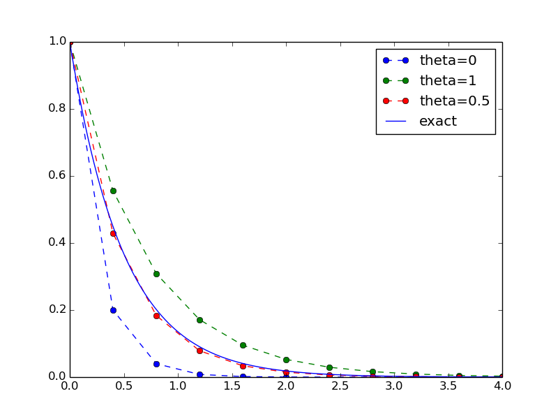
Our example that illustrates the extension is to make a comparison between the numerical solutions for various schemes (\(\theta\) values) and the exact solution:
Wait a minute
Look at the flat program in the section A first, quick implementation, and try to imagine which edits that are required to solve this new problem.
With the solver function at hand, we can simply create a function
with a loop over theta values and add the necessary plot statements:
def experiment_compare_schemes():
    """Compare theta=0,1,0.5 in the same plot."""
    I = 1;  a = 2;  T = 4;  dt = 0.4
    legends = []
    for theta in [0, 1, 0.5]:
        u, t = solver(I, a, T, dt, theta)
        plt.plot(t, u, '--o')
        legends.append('theta=%g' % theta)
    t_e = np.linspace(0, T, 1001)        # very fine mesh for u_e
    u_e = u_exact(t_e, I, a)
    plt.plot(t_e, u_e, 'b-')
    legends.append('exact')
    plt.legend(legends, loc='upper right')
    plotfile = 'tmp'
    plt.savefig(plotfile + '.png');  plt.savefig(plotfile + '.pdf')
A call to this experiment_compare_schemes function must be placed
in the test block, or you can run the program from IPython instead:
In[1]: from decay import *

In[2]: experiment_compare_schemes()
We do not present how the flat program from
the section A more decent program must be refactored to produce the
desired plots, but simply state that the danger of introducing bugs
is significantly larger than when just writing an additional function
in the decay module.
Documenting functions and modules
We have already emphasized the importance of documenting functions with
a doc string (see the section Implementing the numerical algorithm in a function). Now it is time
to show how doc strings should be structured in order to take advantage
of the documentation utilities in the numpy module. The idea is
to follow a convention that in itself makes a good pure text doc string
in the terminal window
and at the same time can be translated to beautiful HTML manuals for
the web.
The conventions for numpy style doc strings are well
documented, so here we just present a basic example that the reader can adopt.
Input arguments to a function are listed under the heading Parameters,
while returned values are listed under Returns. It is a good idea to
also add an Examples section on the usage of the function.
More complicated software may have additional sections, see pydoc numpy.load
for an example. The markup language available for doc strings is
Sphinx-extended reStructuredText. The example below shows typical
constructs: 1) how inline
mathematics is written with the :math: directive, 2) how arguments
to the functions are referred to using single backticks
(inline monospace font for code applies double backticks), and 3) how
arguments and return values are listed with types and explanation.
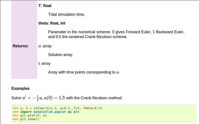
def solver(I, a, T, dt, theta):
    """
    Solve  \( u'=-au \)  with  \( u(0)=I \)  for  \( t \in (0,T] \)
    with steps of `dt` and the method implied by `theta`.

    Parameters
    ----------
    I: float
        Initial condition.
    a: float
        Parameter in the differential equation.
    T: float
        Total simulation time.
    theta: float, int
        Parameter in the numerical scheme. 0 gives
        Forward Euler, 1 Backward Euler, and 0.5
        the centered Crank-Nicolson scheme.

    Returns
    -------
    `u`: array
        Solution array.
    `t`: array
        Array with time points corresponding to `u`.

    Examples
    --------
    Solve  \( u' = -\\frac{1}{2}u, u(0)=1.5 \)
    with the Crank-Nicolson method:

    >>> u, t = solver(I=1.5, a=0.5, T=9, theta=0.5)
    >>> import matplotlib.pyplot as plt
    >>> plt.plot(t, u)
    >>> plt.show()
    """
If you follow such doc string conventions in your software, you can easily produce nice manuals that meet the standard expected within the Python scientific computing community.
Sphinx requires quite a number of manual steps to
prepare a manual, so it is
recommended to use a premade script to automate the steps. (By default,
the script generates documentation for all *.py files in the
current directory.
You need to do a pip install of sphinx and numpydoc to make the
script work.)
Figure Example on Sphinx API manual in HTML provides an example of what
the above doc strings look like when Sphinx has transformed them to HTML.
Example on Sphinx API manual in HTML
Logging intermediate results
Sometimes one may wish that a simulation program could write out
intermediate results for inspection. This could be accomplished by
a (global) verbose variable and code like
if verbose >= 2:
    print 'u[%d]=%g' % (i, u[i])
The professional way to do report intermediate results and problems is, however, to use a logger. This is an object that writes messages to a log file. The messages are classified as debug, info, and warning.
Introductory example
Here is a simple example using defining a logger, using Python’s logging
module:
import logging
# Configure logger
logging.basicConfig(
    filename='myprog.log', filemode='w', level=logging.WARNING,
    format='%(asctime)s - %(levelname)s - %(message)s',
    datefmt='%m/%d/%Y %I:%M:%S %p')
# Perform logging
logging.info('Here is some general info.')
logging.warning('Here is a warning.')
logging.debug('Here is some debugging info.')
logging.critical('Dividing by zero!')
logging.error('Encountered an error.')
Running this program gives the following output in the log file myprog.log:
09/26/2015 09:25:10 AM - INFO - Here is some general info.
09/26/2015 09:25:10 AM - WARNING - Here is a warning.
09/26/2015 09:25:10 AM - CRITICAL - Dividing by zero!
09/26/2015 09:25:10 AM - ERROR - Encountered an error.
The logger has different levels of messages, ordered as
critical, error, warning, info, and debug.
The level argument to logging.basicConfig sets the level
and thereby determines what the logger will print to the file:
all messages at the specified and lower levels are printed.
For example, in the above example we set the level to be
info, and therefore the critical, error, warning, and info
messages were printed, but not the debug message.
Setting level to debug (logging.DEBUG) prints all messages,
while level critical prints only the critical messages.
The filemode argument is set to w such that any existing
log file is overwritten (the default is a, which means append
new messages to an existing log file, but this is seldom what
you want in mathematical computations).
The messages are preceded by the date and time and the level of
the message. This output is governed by the format argument:
asctime is the date and time, levelname is the name of
the message level, and message is the message itself.
Setting format='%(message)s' ensures that just the message and
nothing more is printed on each line. The datefmt string
specifies the formatting of the date and time, using the
rules of the time.strftime function.
Using a logger in our solver function
Let us let a logger write out intermediate results and some debugging
results in the solver function. Such messages are useful for
monitoring the simulation and for debugging it, respectively.
def solver_with_logging(I, a, T, dt, theta):
    """Solve u'=-a*u, u(0)=I, for t in (0,T] with steps of dt."""
    dt = float(dt)               # avoid integer division
    Nt = int(round(T/dt))        # no of time intervals
    T = Nt*dt                    # adjust T to fit time step dt
    u = np.zeros(Nt+1)           # array of u[n] values
    t = np.linspace(0, T, Nt+1)  # time mesh
    logging.debug('solver: dt=%g, Nt=%g, T=%g' % (dt, Nt, T))

    u[0] = I                  # assign initial condition
    for n in range(0, Nt):    # n=0,1,...,Nt-1
        u[n+1] = (1 - (1-theta)*a*dt)/(1 + theta*dt*a)*u[n]

        logging.info('u[%d]=%g' % (n, u[n]))
        logging.debug('1 - (1-theta)*a*dt: %g, %s' %
                      (1-(1-theta)*a*dt,
                       str(type(1-(1-theta)*a*dt))[7:-2]))
        logging.debug('1 + theta*dt*a: %g, %s' %
                      (1 + theta*dt*a,
                       str(type(1 + theta*dt*a))[7:-2]))
    return u, t

def configure_basic_logger():
    logging.basicConfig(
        filename='decay.log', filemode='w', level=logging.DEBUG,
        format='%(asctime)s - %(levelname)s - %(message)s',
        datefmt='%Y.%m.%d %I:%M:%S %p')

import sys

def read_command_line_positional():
    if len(sys.argv) < 6:
        print 'Usage: %s I a T on/off BE/FE/CN dt1 dt2 dt3 ...' % \
              sys.argv[0]; sys.exit(1)  # abort

    I = float(sys.argv[1])
    a = float(sys.argv[2])
    T = float(sys.argv[3])

    # Name of schemes: BE (Backward Euler), FE (Forward Euler),
    # CN (Crank-Nicolson)
    scheme = sys.argv[4]
    scheme2theta = {'BE': 1, 'CN': 0.5, 'FE': 0}
    if scheme in scheme2theta:
        theta = scheme2theta[scheme]
    else:
        print 'Invalid scheme name:', scheme; sys.exit(1)

    dt_values = [float(arg) for arg in sys.argv[5:]]

    return I, a, T, theta, dt_values

def define_command_line_options():
    import argparse
    parser = argparse.ArgumentParser()
    parser.add_argument(
        '--I', '--initial_condition', type=float,
        default=1.0, help='initial condition, u(0)',
        metavar='I')
    parser.add_argument(
        '--a', type=float, default=1.0,
        help='coefficient in ODE', metavar='a')
    parser.add_argument(
        '--T', '--stop_time', type=float,
        default=1.0, help='end time of simulation',
        metavar='T')
    parser.add_argument(
        '--scheme', type=str, default='CN',
        help='FE, BE, or CN')
    parser.add_argument(
        '--dt', '--time_step_values', type=float,
        default=[1.0], help='time step values',
        metavar='dt', nargs='+', dest='dt_values')
    return parser

def read_command_line_argparse():
    parser = define_command_line_options()
    args = parser.parse_args()
    scheme2theta = {'BE': 1, 'CN': 0.5, 'FE': 0}
    data = (args.I, args.a, args.T, scheme2theta[args.scheme],
            args.dt_values)
    return data

def experiment_compare_dt(option_value_pairs=False):
    I, a, T, theta, dt_values = \
       read_command_line_argparse() if option_value_pairs else \
       read_command_line_positional()

    legends = []
    for dt in dt_values:
        u, t = solver(I, a, T, dt, theta)
        plt.plot(t, u)
        legends.append('dt=%g' % dt)
    t_e = np.linspace(0, T, 1001)       # very fine mesh for u_e
    u_e = u_exact(t_e, I, a)
    plt.plot(t_e, u_e, '--')
    legends.append('exact')
    plt.legend(legends, loc='upper right')
    plt.title('theta=%g' % theta)
    plotfile = 'tmp'
    plt.savefig(plotfile + '.png');  plt.savefig(plotfile + '.pdf')

def compute4web(I, a, T, dt, theta=0.5):
    """
    Run a case with the solver, compute error measure,
    and plot the numerical and exact solutions in a PNG
    plot whose data are embedded in an HTML image tag.
    """
    u, t = solver(I, a, T, dt, theta)
    u_e = u_exact(t, I, a)
    e = u_e - u
    E = np.sqrt(dt*np.sum(e**2))

    plt.figure()
    t_e = np.linspace(0, T, 1001)    # fine mesh for u_e
    u_e = u_exact(t_e, I, a)
    plt.plot(t,   u,   'r--o')
    plt.plot(t_e, u_e, 'b-')
    plt.legend(['numerical', 'exact'])
    plt.xlabel('t')
    plt.ylabel('u')
    plt.title('theta=%g, dt=%g' % (theta, dt))
    # Save plot to HTML img tag with PNG code as embedded data
    from parampool.utils import save_png_to_str
    html_text = save_png_to_str(plt, plotwidth=400)

    return E, html_text

def main_GUI(I=1.0, a=.2, T=4.0,
             dt_values=[1.25, 0.75, 0.5, 0.1],
             theta_values=[0, 0.5, 1]):
    # Build HTML code for web page. Arrange plots in columns
    # corresponding to the theta values, with dt down the rows
    theta2name = {0: 'FE', 1: 'BE', 0.5: 'CN'}
    html_text = '<table>\n'
    for dt in dt_values:
        html_text += '<tr>\n'
        for theta in theta_values:
            E, html = compute4web(I, a, T, dt, theta)
            html_text += """
<td>
<center><b>%s, dt=%g, error: %.3E</b></center><br>
%s
</td>
""" % (theta2name[theta], dt, E, html)
        html_text += '</tr>\n'
    html_text += '</table>\n'
    return html_text

def solver_with_doctest(I, a, T, dt, theta):
    """
    Solve u'=-a*u, u(0)=I, for t in (0,T] with steps of dt.


    >>> u, t = solver(I=0.8, a=1.2, T=1.5, dt=0.5, theta=0.5)
    >>> for n in range(len(t)):
    ...     print 't=%.1f, u=%.14f' % (t[n], u[n])
    t=0.0, u=0.80000000000000
    t=0.5, u=0.43076923076923
    t=1.0, u=0.23195266272189
    t=1.5, u=0.12489758761948
    """
    dt = float(dt)               # avoid integer division
    Nt = int(round(T/dt))        # no of time intervals
    T = Nt*dt                    # adjust T to fit time step dt
    u = np.zeros(Nt+1)           # array of u[n] values
    t = np.linspace(0, T, Nt+1)  # time mesh

    u[0] = I                  # assign initial condition
    for n in range(0, Nt):    # n=0,1,...,Nt-1
        u[n+1] = (1 - (1-theta)*a*dt)/(1 + theta*dt*a)*u[n]
    return u, t

def third(x):
    return x/3.

def test_third():
    x = 0.15
    expected = (1/3.)*x
    computed = third(x)
    tol = 1E-15
    success = abs(expected - computed) < tol
    assert success

def u_discrete_exact(n, I, a, theta, dt):
    """Return exact discrete solution of the numerical schemes."""
    dt = float(dt)  # avoid integer division
    A = (1 - (1-theta)*a*dt)/(1 + theta*dt*a)
    return I*A**n

def test_u_discrete_exact():
    """Check that solver reproduces the exact discr. sol."""
    theta = 0.8; a = 2; I = 0.1; dt = 0.8
    Nt = int(8/dt)  # no of steps
    u, t = solver(I=I, a=a, T=Nt*dt, dt=dt, theta=theta)

    # Evaluate exact discrete solution on the mesh
    u_de = np.array([u_discrete_exact(n, I, a, theta, dt)
                     for n in range(Nt+1)])

    # Find largest deviation
    diff = np.abs(u_de - u).max()
    tol = 1E-14
    success = diff < tol
    assert success

def test_potential_integer_division():
    """Choose variables that can trigger integer division."""
    theta = 1; a = 1; I = 1; dt = 2
    Nt = 4
    u, t = solver(I=I, a=a, T=Nt*dt, dt=dt, theta=theta)
    u_de = np.array([u_discrete_exact(n, I, a, theta, dt)
                     for n in range(Nt+1)])
    diff = np.abs(u_de - u).max()
    assert diff < 1E-14

def test_read_command_line_positional():
    # Decide on a data set of input parameters
    I = 1.6;  a = 1.8;  T = 2.2;  theta = 0.5
    dt_values = [0.1, 0.2, 0.05]
    # Expected return from read_command_line_positional
    expected = [I, a, T, theta, dt_values]
    # Construct corresponding sys.argv array
    sys.argv = [sys.argv[0], str(I), str(a), str(T), 'CN'] + \
               [str(dt) for dt in dt_values]
    computed = read_command_line_positional()
    for expected_arg, computed_arg in zip(expected, computed):
        assert expected_arg == computed_arg

def test_read_command_line_argparse():
    I = 1.6;  a = 1.8;  T = 2.2;  theta = 0.5
    dt_values = [0.1, 0.2, 0.05]
    # Expected return from read_command_line_argparse
    expected = [I, a, T, theta, dt_values]
    # Construct corresponding sys.argv array
    command_line = '%s --a %s --I %s --T %s --scheme CN --dt ' % \
                   (sys.argv[0], a, I, T)
    command_line += ' '.join([str(dt) for dt in dt_values])
    sys.argv = command_line.split()
    computed = read_command_line_argparse()
    for expected_arg, computed_arg in zip(expected, computed):
        assert expected_arg == computed_arg

# Classes

class Problem(object):
    def __init__(self, I=1, a=1, T=10):
        self.T, self.I, self.a = I, float(a), T

    def define_command_line_options(self, parser=None):
        """Return updated (parser) or new ArgumentParser object."""
        if parser is None:
            import argparse
            parser = argparse.ArgumentParser()

        parser.add_argument(
            '--I', '--initial_condition', type=float,
            default=1.0, help='initial condition, u(0)',
            metavar='I')
        parser.add_argument(
            '--a', type=float, default=1.0,
            help='coefficient in ODE', metavar='a')
        parser.add_argument(
            '--T', '--stop_time', type=float,
            default=1.0, help='end time of simulation',
            metavar='T')
        return parser

    def init_from_command_line(self, args):
        """Load attributes from ArgumentParser into instance."""
        self.I, self.a, self.T = args.I, args.a, args.T

    def u_exact(self, t):
        """Return the exact solution u(t)=I*exp(-a*t)."""
        I, a = self.I, self.a
        return I*exp(-a*t)


class Solver(object):
    def __init__(self, problem, dt=0.1, theta=0.5):
        self.problem = problem
        self.dt, self.theta = float(dt), theta

    def define_command_line_options(self, parser):
        """Return updated (parser) or new ArgumentParser object."""
        parser.add_argument(
            '--scheme', type=str, default='CN',
            help='FE, BE, or CN')
        parser.add_argument(
            '--dt', '--time_step_values', type=float,
            default=[1.0], help='time step values',
            metavar='dt', nargs='+', dest='dt_values')
        return parser

    def init_from_command_line(self, args):
        """Load attributes from ArgumentParser into instance."""
        self.dt, self.theta = args.dt, args.theta

    def solve(self):
        self.u, self.t = solver(
            self.problem.I, self.problem.a, self.problem.T,
            self.dt, self.theta)

    def error(self):
        """Return norm of error at the mesh points."""
        u_e = self.problem.u_exact(self.t)
        e = u_e - self.u
        E = np.sqrt(self.dt*np.sum(e**2))
        return E

def experiment_classes():
    problem = Problem()
    solver = Solver(problem)

    # Read input from the command line
    parser = problem.define_command_line_options()
    parser = solver. define_command_line_options(parser)
    args = parser.parse_args()
    problem.init_from_command_line(args)
    solver. init_from_command_line(args)

    # Solve and plot
    solver.solve()
    import matplotlib.pyplot as plt
    t_e = np.linspace(0, T, 1001)    # very fine mesh for u_e
    u_e = problem.u_exact(t_e)
    print 'Error:', solver.error()

    plt.plot(t,   u,   'r--o')
    plt.plot(t_e, u_e, 'b-')
    plt.legend(['numerical, theta=%g' % theta, 'exact'])
    plt.xlabel('t')
    plt.ylabel('u')
    plotfile = 'tmp'
    plt.savefig(plotfile + '.png');  plt.savefig(plotfile + '.pdf')
    plt.show()

if __name__ == '__main__':
    configure_logger()
    experiment_compare_dt(True)
    plt.show()
The application code that calls solver_with_logging needs to configure
the logger. The decay module offers a default configure function:
import logging

def configure_basic_logger():
    logging.basicConfig(
        filename='decay.log', filemode='w', level=logging.DEBUG,
        format='%(asctime)s - %(levelname)s - %(message)s',
        datefmt='%Y.%m.%d %I:%M:%S %p')
If the user of a library does not configure a logger or call this configure function, the library should prevent error messages by declaring a default logger that does nothing:
import logging
logging.getLogger('decay').addHandler(logging.NullHandler())
We can run the new solver function with logging in a shell:
>>> import decay
>>> decay.configure_basic_logger()
>>> u, t = decay.solver_with_logging(I=1, a=0.5, T=10, \
           dt=0.5, theta=0.5)
During this execution, each logging message is appended to the log file.
Suppose we add some pause (time.sleep(2)) at each time level such that
the execution takes some time. In another terminal window we can then
monitor the evolution of decay.log and the simulation
by the tail -f Unix command:
Terminal> tail -f decay.log
2015.09.26 05:37:41 AM - INFO - u[0]=1
2015.09.26 05:37:41 AM - INFO - u[1]=0.777778
2015.09.26 05:37:41 AM - INFO - u[2]=0.604938
2015.09.26 05:37:41 AM - INFO - u[3]=0.470508
2015.09.26 05:37:41 AM - INFO - u[4]=0.36595
2015.09.26 05:37:41 AM - INFO - u[5]=0.284628
Especially in simulation where each time step demands considerable CPU time (minutes, hours), it can be handy to monitor such a log file to see the evolution of the simulation.
If we want to look more closely into the numerator and denominator of
the formula for \(u^{n+1}\), we can change the logging level to
level=logging.DEBUG and get output in decay.log like
2015.09.26 05:40:01 AM - DEBUG - solver: dt=0.5, Nt=20, T=10
2015.09.26 05:40:01 AM - INFO - u[0]=1
2015.09.26 05:40:01 AM - DEBUG - 1 - (1-theta)*a*dt: 0.875, float
2015.09.26 05:40:01 AM - DEBUG - 1 + theta*dt*a: 1.125, float
2015.09.26 05:40:01 AM - INFO - u[1]=0.777778
2015.09.26 05:40:01 AM - DEBUG - 1 - (1-theta)*a*dt: 0.875, float
2015.09.26 05:40:01 AM - DEBUG - 1 + theta*dt*a: 1.125, float
2015.09.26 05:40:01 AM - INFO - u[2]=0.604938
2015.09.26 05:40:01 AM - DEBUG - 1 - (1-theta)*a*dt: 0.875, float
2015.09.26 05:40:01 AM - DEBUG - 1 + theta*dt*a: 1.125, float
2015.09.26 05:40:01 AM - INFO - u[3]=0.470508
2015.09.26 05:40:01 AM - DEBUG - 1 - (1-theta)*a*dt: 0.875, float
2015.09.26 05:40:01 AM - DEBUG - 1 + theta*dt*a: 1.125, float
2015.09.26 05:40:01 AM - INFO - u[4]=0.36595
2015.09.26 05:40:01 AM - DEBUG - 1 - (1-theta)*a*dt: 0.875, float
2015.09.26 05:40:01 AM - DEBUG - 1 + theta*dt*a: 1.125, float
Logging can be much more sophisticated than shown above. One can, e.g., output critical messages to the screen and all messages to a file. This requires more code as demonstrated in the Logging Cookbook.
User interfaces
It is good programming practice to let programs read input from some user interface, rather than requiring users to edit parameter values in the source code. With effective user interfaces it becomes easier and safer to apply the code for scientific investigations and in particular to automate large-scale investigations by other programs (see the section Automating scientific experiments).
Reading input data can be done in many ways. We have to decide on the functionality of the user interface, i.e., how we want to operate the program when providing input. Thereafter, we use appropriate tools to implement the particular user interface. There are four basic types of user interface, listed here according to implementational complexity, from lowest to highest:
- Questions and answers in the terminal window
- Command-line arguments
- Reading data from files
- Graphical user interfaces (GUIs)
Personal preferences of user interfaces differ substantially, and it is
difficult to present recommendations or pros and cons.
Alternatives 2 and 4 are most popular and will be addressed next.
The goal is to make it easy for the user to
set physical and numerical parameters in
our decay.py program. However, we use a little toy program, called
prog.py, as introductory
example:
delta = 0.5
p = 2
from math import exp
result = delta*exp(-p)
print result
The essential content is that prog.py has two input parameters: delta
and p. A user interface will replace the first two assignments to
delta and p.
Command-line arguments
The command-line arguments are all the words that appear on the
command line after the program name. Running a program prog.py
as python prog.py arg1 arg2 means that there are two command-line arguments
(separated by white space): arg1 and arg2.
Python stores all command-line arguments in
a special list sys.argv. (The name argv stems from the C language and
stands for “argument values”. In C there is also an integer variable
called argc reflecting the number of arguments, or “argument counter”.
A lot of programming languages have adopted the variable name argv for
the command-line arguments.)
Here is an example on a
program what_is_sys_argv.py that can show us what the command-line arguments
are
import sys
print sys.argv
A sample run goes like
Terminal> python what_is_sys_argv.py 5.0 'two words' -1E+4
['what_is_sys_argv.py', '5.0', 'two words', '-1E+4']
We make two observations:
sys.argv[0]is the name of the program, and the sublistsys.argv[1:]contains all the command-line arguments.- Each command-line argument is available as a string. A conversion to
floatis necessary if we want to compute with the numbers 5.0 and \(10^4\).
There are, in principle, two ways of programming with command-line arguments in Python:
- Positional arguments: Decide upon a sequence of parameters on the command line and read their values directly from the
sys.argv[1:]list.- Option-value pairs: Use
--option valueon the command line to replace the default value of an input parameteroptionbyvalue(and utilize theargparse.ArgumentParsertool for implementation).
Suppose we want to run some program prog.py with
specification of two parameters p and delta on the command line.
With positional command-line arguments we write
Terminal> python prog.py 2 0.5
and must know that the first argument 2 represents p and the
next 0.5 is the value of delta.
With option-value pairs we can run
Terminal> python prog.py --delta 0.5 --p 2
Now, both p and delta are supposed to have default values in the program,
so we need to specify only the parameter that is to be changed from
its default value, e.g.,
Terminal> python prog.py --p 2         # p=2, default delta
Terminal> python prog.py --delta 0.7   # delta-0.7, default a
Terminal> python prog.py               # default a and delta
How do we extend the prog.py code for positional arguments
and option-value pairs? Positional arguments require very simple
code:
import sys
p = float(sys.argv[1])
delta = float(sys.argv[2])

from math import exp
result = delta*exp(-p)
print result
If the user forgets to supply two command-line arguments, Python will
raise an IndexError exception and produce a long error message.
To avoid that, we should use a try-except construction:
import sys
try:
    p = float(sys.argv[1])
    delta = float(sys.argv[2])
except IndexError:
    print 'Usage: %s p delta' % sys.argv[0]
    sys.exit(1)

from math import exp
result = delta*exp(-p)
print result
Using sys.exit(1) aborts the program. The value 1 (actually any
value different from 0) notifies the operating system that the
program failed.
Command-line arguments are strings
Note that all elements in sys.argv are string objects.
If the values are used in mathematical computations, we need
to explicitly convert the strings to numbers.
Option-value pairs requires more programming and is actually
better explained in a more comprehensive example below.
Minimal code for our prog.py program reads
import argparse
parser = argparse.ArgumentParser()
parser.add_argument('--p', default=1.0)
parser.add_argument('--delta', default=0.1)

args = parser.parse_args()
p = args.p
delta = args.delta

from math import exp
result = delta*exp(-p)
print result
Because the default values of delta and p are float numbers,
the args.delta and args.p variables are automatically of type float.
Our next task is to use these basic code constructs to equip our
decay.py module with command-line interfaces.
Positional command-line arguments
For our decay.py module file, we want to include functionality such
that we can read \(I\), \(a\), \(T\), \(\theta\), and a range of \(\Delta t\)
values from the command line. A plot is then to be made, comparing
the different numerical solutions for different \(\Delta t\) values
against the exact solution. The technical details of getting the
command-line information into the program is covered in the next
two sections.
The simplest way of reading the input parameters is to
decide on their sequence on the command line and just index
the sys.argv list accordingly.
Say the sequence of input data for some functionality in
decay.py is \(I\), \(a\), \(T\), \(\theta\) followed by an
arbitrary number of \(\Delta t\) values. This code extracts
these positional command-line arguments:
def read_command_line_positional():
    if len(sys.argv) < 6:
        print 'Usage: %s I a T on/off BE/FE/CN dt1 dt2 dt3 ...' % \
              sys.argv[0]; sys.exit(1)  # abort

    I = float(sys.argv[1])
    a = float(sys.argv[2])
    T = float(sys.argv[3])
    theta = float(sys.argv[4])
    dt_values = [float(arg) for arg in sys.argv[5:]]

    return I, a, T, theta, dt_values
Note that we may use a try-except construction instead of the if test.
A run like
Terminal> python decay.py 1 0.5 4 0.5 1.5 0.75 0.1
results in
sys.argv = ['decay.py', '1', '0.5', '4', '0.5', '1.5', '0.75', '0.1']
and consequently the assignments I=1.0, a=0.5, T=4.0, thet=0.5,
and dt_values = [1.5, 0.75, 0.1].
Instead of specifying the \(\theta\) value, we could be a bit more
sophisticated and let the user write the name of the scheme:
BE for Backward Euler, FE for Forward Euler, and CN
for Crank-Nicolson. Then we must map this string to the proper
\(\theta\) value, an operation elegantly done by a dictionary:
scheme = sys.argv[4]
scheme2theta = {'BE': 1, 'CN': 0.5, 'FE': 0}
if scheme in scheme2theta:
    theta = scheme2theta[scheme]
else:
    print 'Invalid scheme name:', scheme; sys.exit(1)
Now we can do
Terminal> python decay.py 1 0.5 4 CN 1.5 0.75 0.1
and get `theta=0.5`in the code.
Option-value pairs on the command line
Now we want to specify option-value pairs on the command line,
using --I for I (\(I\)), --a for a (\(a\)), --T for T (\(T\)),
--scheme for the scheme name (BE, FE, CN),
and --dt for the sequence of dt (\(\Delta t\)) values.
Each parameter must have a sensible default value so
that we specify the option on the command line only when the default
value is not suitable. Here is a typical run:
Terminal> python decay.py --I 2.5 --dt 0.1 0.2 0.01 --a 0.4
Observe the major advantage over positional command-line arguments: the input is much easier to read and much easier to write. With positional arguments it is easy to mess up the sequence of the input parameters and quite challenging to detect errors too, unless there are just a couple of arguments.
Python’s ArgumentParser tool in the argparse module makes it easy
to create a professional command-line interface to any program. The
documentation of ArgumentParser demonstrates its
versatile applications, so we shall here just list an example
containing the most basic features. It always pays off to use ArgumentParser
rather than trying to manually inspect and interpret option-value pairs
in sys.argv!
The use of ArgumentParser typically involves three steps:
import argparse
parser = argparse.ArgumentParser()

# Step 1: add arguments
parser.add_argument('--option_name', ...)

# Step 2: interpret the command line
args = parser.parse_args()

# Step 3: extract values
value = args.option_name
A function for setting up all the options is handy:
def define_command_line_options():
    import argparse
    parser = argparse.ArgumentParser()
    parser.add_argument(
        '--I', '--initial_condition', type=float,
        default=1.0, help='initial condition, u(0)',
        metavar='I')
    parser.add_argument(
        '--a', type=float, default=1.0,
        help='coefficient in ODE', metavar='a')
    parser.add_argument(
        '--T', '--stop_time', type=float,
        default=1.0, help='end time of simulation',
        metavar='T')
    parser.add_argument(
        '--scheme', type=str, default='CN',
        help='FE, BE, or CN')
    parser.add_argument(
        '--dt', '--time_step_values', type=float,
        default=[1.0], help='time step values',
        metavar='dt', nargs='+', dest='dt_values')
    return parser
Each command-line option is defined through the parser.add_argument
method [1]. Alternative options, like the short --I and the more
explaining version --initial_condition can be defined. Other arguments
are type for the Python object type, a default value, and a help
string, which gets printed if the command-line argument -h or --help is
included. The metavar argument specifies the value associated with
the option when the help string is printed. For example, the option for
\(I\) has this help output:
Terminal> python decay.py -h
  ...
  --I I, --initial_condition I
                        initial condition, u(0)
  ...
The structure of this output is
--I metavar, --initial_condition metavar
                      help-string
| [1] | We use the expression method here, because parser
is a class variable and functions in classes are known as methods in Python
and many other languages.
Readers not familiar with class programming can just substitute
this use of method by function. |
Finally, the --dt option demonstrates how to allow for more than one
value (separated by blanks) through the nargs='+' keyword argument.
After the command line is parsed, we get an object where the values of
the options are stored as attributes. The attribute name is specified
by the dist keyword argument, which for the --dt option is
dt_values. Without the dest argument, the value of an option --opt
is stored as the attribute opt.
The code below demonstrates how to read the command line and extract the values for each option:
def read_command_line_argparse():
    parser = define_command_line_options()
    args = parser.parse_args()
    scheme2theta = {'BE': 1, 'CN': 0.5, 'FE': 0}
    data = (args.I, args.a, args.T, scheme2theta[args.scheme],
            args.dt_values)
    return data
As seen, the values of the command-line options are available as
attributes in args: args.opt holds the value of option --opt, unless
we used the dest argument (as for --dt_values) for specifying the
attribute name. The args.opt attribute has the object type specified
by type (str by default).
The making of the plot is not dependent on whether we read data from the command line as positional arguments or option-value pairs:
def experiment_compare_dt(option_value_pairs=False):
    I, a, T, theta, dt_values = \
       read_command_line_argparse() if option_value_pairs else \
       read_command_line_positional()

    legends = []
    for dt in dt_values:
        u, t = solver(I, a, T, dt, theta)
        plt.plot(t, u)
        legends.append('dt=%g' % dt)
    t_e = np.linspace(0, T, 1001)       # very fine mesh for u_e
    u_e = u_exact(t_e, I, a)
    plt.plot(t_e, u_e, '--')
    legends.append('exact')
    plt.legend(legends, loc='upper right')
    plt.title('theta=%g' % theta)
    plotfile = 'tmp'
    plt.savefig(plotfile + '.png');  plt.savefig(plotfile + '.pdf')
Creating a graphical web user interface
The Python package Parampool
can be used to automatically generate a web-based graphical user interface
(GUI) for our simulation program. Although the programming technique
dramatically simplifies the efforts to create a GUI, the forthcoming
material on equipping our decay module with a GUI is quite technical
and of significantly less importance than knowing how to make
a command-line interface.
Making a compute function
The first step is to identify a function that performs the computations and that takes the necessary input variables as arguments. This is called the compute function in Parampool terminology. The purpose of this function is to take values of \(I\), \(a\), \(T\) together with a sequence of \(\Delta t\) values and a sequence of \(\theta\) and plot the numerical against the exact solution for each pair of \((\theta, \Delta t)\). The plots can be arranged as a table with the columns being scheme type (\(\theta\) value) and the rows reflecting the discretization parameter (\(\Delta t\) value). Figure Automatically generated graphical web interface displays what the graphical web interface may look like after results are computed (there are \(3\times 3\) plots in the GUI, but only \(2\times 2\) are visible in the figure).
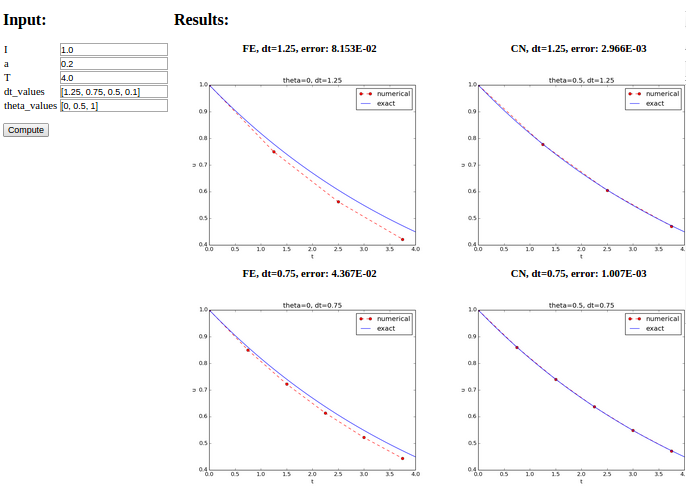
Automatically generated graphical web interface
To tell Parampool what type of input data we have,
we assign default values of the right type to all arguments in the
compute function, here called main_GUI:
def main_GUI(I=1.0, a=.2, T=4.0,
             dt_values=[1.25, 0.75, 0.5, 0.1],
             theta_values=[0, 0.5, 1]):
The compute function must return the HTML code we want for displaying
the result in a web page. Here we want to show a
table of plots.
Assume for now that the HTML code for one plot and the value of the
norm of the error can be computed by some other function compute4web.
The main_GUI function can then loop over \(\Delta t\) and \(\theta\)
values and put each plot in an HTML table. Appropriate code goes like
def main_GUI(I=1.0, a=.2, T=4.0,
             dt_values=[1.25, 0.75, 0.5, 0.1],
             theta_values=[0, 0.5, 1]):
    # Build HTML code for web page. Arrange plots in columns
    # corresponding to the theta values, with dt down the rows
    theta2name = {0: 'FE', 1: 'BE', 0.5: 'CN'}
    html_text = '<table>\n'
    for dt in dt_values:
        html_text += '<tr>\n'
        for theta in theta_values:
            E, html = compute4web(I, a, T, dt, theta)
            html_text += """
<td>
<center><b>%s, dt=%g, error: %.3E</b></center><br>
%s
</td>
""" % (theta2name[theta], dt, E, html)
        html_text += '</tr>\n'
    html_text += '</table>\n'
    return html_text
Making one plot is done in compute4web. The statements should be
straightforward from earlier examples, but there is one new feature:
we use a tool in Parampool to embed the PNG code for a plot file
directly in an HTML image tag. The details are hidden from the
programmer, who can just rely on
relevant HTML code in the string html_text. The function looks like
def compute4web(I, a, T, dt, theta=0.5):
    """
    Run a case with the solver, compute error measure,
    and plot the numerical and exact solutions in a PNG
    plot whose data are embedded in an HTML image tag.
    """
    u, t = solver(I, a, T, dt, theta)
    u_e = u_exact(t, I, a)
    e = u_e - u
    E = np.sqrt(dt*np.sum(e**2))

    plt.figure()
    t_e = np.linspace(0, T, 1001)    # fine mesh for u_e
    u_e = u_exact(t_e, I, a)
    plt.plot(t,   u,   'r--o')
    plt.plot(t_e, u_e, 'b-')
    plt.legend(['numerical', 'exact'])
    plt.xlabel('t')
    plt.ylabel('u')
    plt.title('theta=%g, dt=%g' % (theta, dt))
    # Save plot to HTML img tag with PNG code as embedded data
    from parampool.utils import save_png_to_str
    html_text = save_png_to_str(plt, plotwidth=400)

    return E, html_text
Generating the user interface
The web GUI is automatically generated by the following code, placed in the file decay_GUI_generate.py.
from parampool.generator.flask import generate
from decay import main_GUI
generate(main_GUI,
         filename_controller='decay_GUI_controller.py',
         filename_template='decay_GUI_view.py',
         filename_model='decay_GUI_model.py')
Running the decay_GUI_generate.py program results in three new
files whose names are specified in the call to generate:
decay_GUI_model.pydefines HTML widgets to be used to set input data in the web interface,templates/decay_GUI_views.pydefines the layout of the web page,decay_GUI_controller.pyruns the web application.
We only need to run the last program, and there is no need to look into these files.
Running the web application
The web GUI is started by
Terminal> python decay_GUI_controller.py
Open a web browser at the location 127.0.0.1:5000. Input fields for
I, a, T, dt_values, and theta_values are presented. Figure
Automatically generated graphical web interface shows a part of the resulting page if we run
with the default values for the input parameters.
With the techniques demonstrated here, one can
easily create a tailored web GUI for a particular type of application
and use it to interactively explore physical and numerical effects.
Tests for verifying implementations
Any module with functions should have a set of tests that can check the correctness of the implementations. There exists well-established procedures and corresponding tools for automating the execution of such tests. These tools allow large test sets to be run with a one-line command, making it easy to check that the software still works (as far as the tests can tell!). Here we shall illustrate two important software testing techniques: doctest and unit testing. The first one is Python specific, while unit testing is the dominating test technique in the software industry today.
Doctests
A doc string, the first string after the function header, is used to
document the purpose of functions and their arguments
(see the section Implementing the numerical algorithm in a function). Very often it
is instructive to include an example in the doc string
on how to use the function.
Interactive examples in the Python shell are most illustrative as
we can see the output resulting from the statements and expressions.
For example,
in the solver function, we can include an example on calling
this function and printing the computed u and t arrays:
def solver(I, a, T, dt, theta):
    """
    Solve u'=-a*u, u(0)=I, for t in (0,T] with steps of dt.


    >>> u, t = solver(I=0.8, a=1.2, T=1.5, dt=0.5, theta=0.5)
    >>> for n in range(len(t)):
    ...     print 't=%.1f, u=%.14f' % (t[n], u[n])
    t=0.0, u=0.80000000000000
    t=0.5, u=0.43076923076923
    t=1.0, u=0.23195266272189
    t=1.5, u=0.12489758761948
    """
    ...
When such interactive demonstrations are inserted in doc strings,
Python’s doctest
module can be used to automate running all commands
in interactive sessions and compare new output with the output
appearing in the doc string. All we have to do in the current example
is to run the module file decay.py with
Terminal> python -m doctest decay.py
This command imports the doctest module, which runs all
doctests found in the file and reports discrepancies between
expected and computed output.
Alternatively, the test block in a module may run all doctests
by
if __name__ == '__main__':
    import doctest
    doctest.testmod()
Doctests can also be embedded in nose/pytest unit tests as explained in the next section.
Doctests prevent command-line arguments
No additional command-line argument is allowed when running doctests. If your program relies on command-line input, make sure the doctests can be run without such input on the command line.
However, you can simulate command-line input by filling sys.argv
with values, e.g.,
import sys; sys.argv = '--I 1.0 --a 5'.split()
The execution command above will report any problem if a test fails.
As an illustration, let us alter the u value at t=1.5 in
the output of the doctest by replacing the last digit 8 by 7.
This edit triggers a report:
Terminal> python -m doctest decay.py
********************************************************
File "decay.py", line ...
Failed example:
    for n in range(len(t)):
        print 't=%.1f, u=%.14f' % (t[n], u[n])
Expected:
    t=0.0, u=0.80000000000000
    t=0.5, u=0.43076923076923
    t=1.0, u=0.23195266272189
    t=1.5, u=0.12489758761948
Got:
    t=0.0, u=0.80000000000000
    t=0.5, u=0.43076923076923
    t=1.0, u=0.23195266272189
    t=1.5, u=0.12489758761947
Pay attention to the number of digits in doctest results
Note that in the output of t and u we write u with 14 digits.
Writing all 16 digits is not a good idea: if the tests are run on
different hardware, round-off errors might be different, and
the doctest module detects that the numbers are not precisely the same
and reports failures. In the present application, where \(0 < u(t) \leq 0.8\),
we expect round-off errors to be of size \(10^{-16}\), so comparing 15
digits would probably be reliable, but we compare 14 to be on the
safe side. On the other hand, comparing a small number of digits may
hide software errors.
Doctests are highly encouraged as they do two things: 1) demonstrate how a function is used and 2) test that the function works.
Unit tests and test functions
The unit testing technique consists of identifying smaller units of code and writing one or more tests for each unit. One unit can typically be a function. Each test should, ideally, not depend on the outcome of other tests. The recommended practice is actually to design and write the unit tests first and then implement the functions!
In scientific computing it is not always obvious how to best perform
unit testing. The units are naturally larger than in non-scientific
software. Very often the solution procedure of a mathematical problem
identifies a unit, such as our solver function.
Two Python test frameworks: nose and pytest
Python offers two very easy-to-use software frameworks for implementing unit tests: nose and pytest. These work (almost) in the same way, but our recommendation is to go for pytest.
Test function requirements
For a test to qualify as a test function in nose or pytest, three rules must be followed:
- The function name must start with
test_.- Function arguments are not allowed.
- An
AssertionErrorexception must be raised if the test fails.
A specific example might be illustrative before proceeding. We have the following function that we want to test:
def double(n):
    return 2*n
The corresponding test function could, in principle, have been written as
def test_double():
    """Test that double(n) works for one specific n."""
    n = 4
    expected = 2*4
    computed = double(4)
    if expected != computed:
        raise AssertionError
The last two lines, however, are never written like this in test functions.
Instead, Python’s assert statement is used: assert success, msg, where
success is a boolean variable, which is False if the test fails, and
msg is an optional message string that is printed when the test fails.
A better version of the test function is therefore
def test_double():
    """Test that double(n) works for one specific n."""
    n = 4
    expected = 2*4
    computed = double(4)
    msg = 'expected %g, computed %g' % (expected, computed)
    success = expected == computed
    assert success, msg
Comparison of real numbers
Because of the finite precision arithmetics on a computer, which gives
rise to round-off errors, the == operator is not suitable for
checking whether two real numbers are equal. Obviously, this principle
also applies to tests in test functions.
We must therefore replace a == b by a comparison
based on a tolerance tol: abs(a-b) < tol. The next example illustrates
the problem and its solution.
Here is a slightly different function that we want to test:
def third(x):
    return x/3.
We write a test function where the expected result is computed as \(\frac{1}{3}x\) rather than \(x/3\):
def test_third():
    """Check that third(x) works for many x values."""
    for x in np.linspace(0, 1, 21):
        expected = (1/3.0)*x
        computed = third(x)
        success = expected == computed
        assert success
This test_third function executes silently, i.e., no failure,
until x becomes 0.15. Then round-off errors make the == comparison
False. In fact, seven of the x values above face this problem.
The solution is to compare expected and computed
with a small tolerance:
def test_third():
    """Check that third(x) works for many x values."""
    for x in np.linspace(0, 1, 21):
        expected = (1/3.)*x
        computed = third(x)
        tol = 1E-15
        success = abs(expected - computed) < tol
        assert success
Always compare real numbers with a tolerance
Real numbers should never be compared with the == operator, but always
with the absolute value of the difference and a tolerance.
So, replace a == b, if a and/or b is float, by
tol = 1E-14
abs(a - b) < tol
The suitable size of tol depends on the size of a and b
(see Problem 5.5: Investigate the size of tolerances in comparisons). Unless a and b are around
unity in size, one should use a relative difference:
tol = 1E-14
abs((a - b)/a) < tol
Special assert functions from nose
Test frameworks often contain more tailored
assert functions that can be called instead of using the assert
statement. For example, comparing two objects within
a tolerance, as in the present
case, can be done by the assert_almost_equal from the nose
framework:
import nose.tools as nt

def test_third():
    x = 0.15
    expected = (1/3.)*x
    computed = third(x)
    nt.assert_almost_equal(
        expected, computed, delta=1E-15,
        msg='diff=%.17E' % (expected - computed))
Whether to use the plain assert statement with a comparison based on
a tolerance or to use the ready-made function assert_almost_equal
depends on the programmer’s preference. The examples used in the
documentation of the pytest framework stick to the plain assert
statement.
Locating test functions
Test functions can reside in a module together with the functions they
are supposed to verify, or the test functions can be collected in
separate files having names starting with test. Actually,
nose and pytest can recursively run all test functions
in all test*.py
files in the current directory, as well as in all subdirectories!
The decay.py module file features
test functions in the module, but we could equally well have made
a subdirectory tests and put the test functions in
tests/test_decay.py.
Running tests
To run all test functions in the file decay.py do
Terminal> nosetests -s -v decay.py
Terminal> py.test -s -v decay.py
The -s option ensures that output from the test functions is printed
in the terminal window, while -v prints the outcome of each individual
test function.
Alternatively, if the test functions are located in some separate
test*.py files,
we can just write
Terminal> py.test -s -v
to recursively run all test functions in the current directory tree. The corresponding
Terminal> nosetests -s -v
command does the same, but requires subdirectory names to start
with test or end with _test or _tests (which is a good habit anyway).
An example of a tests directory with a test*.py
file is found in src/softeng/tests.
Embedding doctests in a test function
Doctests can also be executed from nose/pytest unit tests. Here is an
example of a file test_decay_doctest.py where we in the test
block run all the doctests in the imported module decay, but we also
include a local test function that does the same:
import sys, os
sys.path.insert(0, os.pardir)
import decay
import doctest

def test_decay_module_with_doctest():
    """Doctest embedded in a nose/pytest unit test."""
    # Test all functions with doctest in module decay
    failure_count, test_count = doctest.testmod(m=decay)
    assert failure_count == 0

if __name__ == '__main__':
    # Run all functions with doctests in this module
    failure_count, test_count = doctest.testmod(m=decay)
Running this file as a program from the command line
triggers the doctest.testmod call
in the test block, while applying py.test or nosetests to the file triggers
an import of the file and execution of the test function
test_decay_modue_with_doctest.
Installing nose and pytest
With pip available, it is trivial to install nose and/or pytest:
sudo pip install nose and sudo pip install pytest.
Test function for the solver
Finding good test problems for verifying the implementation of numerical methods is a topic on its own. The challenge is that we very seldom know what the numerical errors are. For the present model problem (195)-(196) solved by (197) one can, fortunately, derive a formula for the numerical approximation:
Then we know that the implementation should produce numbers that agree with this formula to machine precision. The formula for \(u^n\) is known as an exact discrete solution of the problem and can be coded as
def u_discrete_exact(n, I, a, theta, dt):
    """Return exact discrete solution of the numerical schemes."""
    dt = float(dt)  # avoid integer division
    A = (1 - (1-theta)*a*dt)/(1 + theta*dt*a)
    return I*A**n
A test function can evaluate this solution on a time mesh
and check that the u values produced by the solver function
do not deviate with more than a small tolerance:
def test_u_discrete_exact():
    """Check that solver reproduces the exact discr. sol."""
    theta = 0.8; a = 2; I = 0.1; dt = 0.8
    Nt = int(8/dt)  # no of steps
    u, t = solver(I=I, a=a, T=Nt*dt, dt=dt, theta=theta)

    # Evaluate exact discrete solution on the mesh
    u_de = np.array([u_discrete_exact(n, I, a, theta, dt)
                     for n in range(Nt+1)])

    # Find largest deviation
    diff = np.abs(u_de - u).max()
    tol = 1E-14
    success = diff < tol
    assert success
Among important things to consider when constructing test functions
is testing the effect of wrong input to the function being tested.
In our solver function, for example, integer values of \(a\), \(\Delta t\), and
\(\theta\) may cause unintended integer
division. We should therefore add a test to make sure our solver
function does not fall into this potential trap:
def test_potential_integer_division():
    """Choose variables that can trigger integer division."""
    theta = 1; a = 1; I = 1; dt = 2
    Nt = 4
    u, t = solver(I=I, a=a, T=Nt*dt, dt=dt, theta=theta)
    u_de = np.array([u_discrete_exact(n, I, a, theta, dt)
                     for n in range(Nt+1)])
    diff = np.abs(u_de - u).max()
    assert diff < 1E-14
In more complicated problems where there is no exact solution of the numerical problem solved by the software, one must use the method of manufactured solutions, compute convergence rates for a series of \(\Delta t\) values, and check that the rates converges to the expected ones (from theory). This type of testing is fully explained in the section Computing convergence rates.
Test function for reading positional command-line arguments
The function read_command_line_positional extracts numbers from the
command line. To test it, we must decide on a set of values for
the input data, fill sys.argv
accordingly, and check that we get the expected values:
def test_read_command_line_positional():
    # Decide on a data set of input parameters
    I = 1.6;  a = 1.8;  T = 2.2;  theta = 0.5
    dt_values = [0.1, 0.2, 0.05]
    # Expected return from read_command_line_positional
    expected = [I, a, T, theta, dt_values]
    # Construct corresponding sys.argv array
    sys.argv = [sys.argv[0], str(I), str(a), str(T), 'CN'] + \
               [str(dt) for dt in dt_values]
    computed = read_command_line_positional()
    for expected_arg, computed_arg in zip(expected, computed):
        assert expected_arg == computed_arg
Note that sys.argv[0] is always the program name and that we have to
copy that string from the original sys.argv array to the new one we
construct in the test function. (Actually, this test function destroys
the original sys.argv that Python fetched from the command line.)
Any numerical code writer should always be skeptical to the use of the exact
equality operator == in test functions, since round-off errors often
come into play. Here, however, we set some real values, convert them
to strings and convert back again to real numbers (of the same precision).
This string-number conversion does not involve any finite precision
arithmetics effects so we
can safely use == in tests. Note also that the last element in
expected and computed is the list dt_values, and == works
for comparing two lists as well.
Test function for reading option-value pairs
The function read_command_line_argparse can be verified with a
test function that has the same setup as test_read_command_line_positional
above.
However, the construction of the command line is a bit more complicated.
We find it convenient to construct the line as a string and then
split the line into words to get the desired list sys.argv:
def test_read_command_line_argparse():
    I = 1.6;  a = 1.8;  T = 2.2;  theta = 0.5
    dt_values = [0.1, 0.2, 0.05]
    # Expected return from read_command_line_argparse
    expected = [I, a, T, theta, dt_values]
    # Construct corresponding sys.argv array
    command_line = '%s --a %s --I %s --T %s --scheme CN --dt ' % \
                   (sys.argv[0], a, I, T)
    command_line += ' '.join([str(dt) for dt in dt_values])
    sys.argv = command_line.split()
    computed = read_command_line_argparse()
    for expected_arg, computed_arg in zip(expected, computed):
        assert expected_arg == computed_arg
Recall that the Python function zip enables iteration over
several lists, tuples, or arrays at the same time.
Let silent test functions speak up during development
When you develop test functions in a module, it is common to use IPython for interactive experimentation:
In[1]: import decay

In[2]: decay.test_read_command_line_argparse()
Note that a working test function is completely silent! Many find it psychologically annoying to convince themselves that a completely silent function is doing the right things. It can therefore, during development of a test function, be convenient to insert print statements in the function to monitor that the function body is indeed executed. For example, one can print the expected and computed values in the terminal window:
def test_read_command_line_argparse():
    ...
    for expected_arg, computed_arg in zip(expected, computed):
        print expected_arg, computed_arg
        assert expected_arg == computed_arg
After performing this edit, we want to run the test again, but in IPython the module must first be reloaded (reimported):
In[3]: reload(decay)  # force new import

In[2]: decay.test_read_command_line_argparse()
1.6 1.6
1.8 1.8
2.2 2.2
0.5 0.5
[0.1, 0.2, 0.05] [0.1, 0.2, 0.05]
Now we clearly see the objects that are compared.
Classical class-based unit testing
The test functions written for the nose and pytest frameworks are
very straightforward and to the point, with no framework-required boilerplate
code. We just write the statements we need to get the computations and
comparisons done, before applying the required assert.
The classical way of implementing unit tests (which derives from the
JUnit object-oriented tool in Java) leads to much more comprehensive
implementations with a lot of boilerplate code. Python comes with a
built-in module unittest for doing this type of classical unit
tests. Although nose or pytest are much more convenient to use than
unittest, class-based unit testing in the style of unittest has a
very strong position in computer science and is so widespread in
the software industry that
even computational scientists should have an idea how such unit test
code is written. A short demo of unittest is therefore included
next. (Readers who are not familiar with object-oriented programming
in Python may find the text hard to understand, but one can safely
jump to the next section.)
Suppose we have a function double(x) in a module file mymod.py:
def double(x):
    return 2*x
Unit testing with the aid of the unittest module
consists of writing a file test_mymod.py for testing the functions
in mymod.py. The individual tests must be methods with names
starting with test_ in a class derived from class TestCase in
unittest. With one test method for the function double, the
test_mymod.py file becomes
import unittest
import mymod

class TestMyCode(unittest.TestCase):
    def test_double(self):
        x = 4
        expected = 2*x
        computed = mymod.double(x)
        self.assertEqual(expected, computed)

if __name__ == '__main__':
    unittest.main()
The test is run by executing the test file test_mymod.py as a standard
Python program. There is no support in unittest for automatically
locating and running all tests in all test files in a directory tree.
We could use the basic assert statement as we did with nose and pytest
functions, but those who write code based on unittest almost
exclusively use the wide range of built-in assert functions such
as assertEqual, assertNotEqual, assertAlmostEqual, to mention
some of them.
Translation of the test functions from the previous sections
to unittest means making a new file test_decay.py file with a
test class TestDecay where the stand-alone functions for
nose/pytest now become methods in this class.
import unittest
import decay
import numpy as np

def u_discrete_exact(n, I, a, theta, dt):
    ...

class TestDecay(unittest.TestCase):

    def test_exact_discrete_solution(self):
        theta = 0.8; a = 2; I = 0.1; dt = 0.8
        Nt = int(8/dt)  # no of steps
        u, t = decay.solver(I=I, a=a, T=Nt*dt, dt=dt, theta=theta)
        # Evaluate exact discrete solution on the mesh
        u_de = np.array([u_discrete_exact(n, I, a, theta, dt)
                         for n in range(Nt+1)])
        diff = np.abs(u_de - u).max()  # largest deviation
        self.assertAlmostEqual(diff, 0, delta=1E-14)

    def test_potential_integer_division(self):
        ...
        self.assertAlmostEqual(diff, 0, delta=1E-14)

    def test_read_command_line_positional(self):
        ...
        for expected_arg, computed_arg in zip(expected, computed):
            self.assertEqual(expected_arg, computed_arg)

    def test_read_command_line_argparse(self):
        ...

if __name__ == '__main__':
    unittest.main()
Sharing the software with other users
As soon as you have some working software that you intend to share with others, you should package your software in a standard way such that users can easily download your software, install it, improve it, and ask you to approve their improvements in new versions of the software. During recent years, the software development community has established quite firm tools and rules for how all this is done. The following subsections cover three steps in sharing software:
- Organizing the software for public distribution.
- Uploading the software to a cloud service (here GitHub).
- Downloading and installing the software.
Organizing the software directory tree
We start with organizing our software as a directory tree. Our
software consists of one module file, decay.py, and possibly some
unit tests in a separate file located in a directory tests.
The decay.py can be used as a module or as a program. For distribution
to other users who install the program decay.py in system directories,
we need to insert the following line at the top of the file:
#!/usr/bin/env python
This line makes it possible to write just the filename and get the
file executed by the python program (or more precisely, the first
python program found in the directories in the PATH environment
variable).
Distributing just a module file
Let us start out with the minimum solution alternative: distributing
just the decay.py file. Then the software is just one file and all
we need is a directory with this file. This directory will also
contain an installation script setup.py and a README file
telling what the software is about, the author’s email address, a URL
for downloading the software, and other useful information.
The setup.py file can be as short as
from distutils.core import setup
setup(name='decay',
      version='0.1',
      py_modules=['decay'],
      scripts=['decay.py'],
      )
The py_modules argument specifies a list of modules to be installed, while
scripts specifies stand-alone programs. Our decay.py can be used
either as a module or as an executable program, so we want users to
have both possibilities.
Distributing a package
If the software consists of more files than one or two modules, one
should make a Python package out of it. In our case we make a
package decay containing one module, also called decay.
To make a package decay, create a directory decay and an empty
file in it with name __init__.py.
A setup.py script must now specify the directory name of the package
and also an executable program (scripts=)
in case we want to run decay.py as a stand-alone application:
from distutils.core import setup
import os

setup(name='decay',
      version='0.1',
      author='Hans Petter Langtangen',
      author_email='hpl@simula.no',
      url='https://github.com/hplgit/decay-package/',
      packages=['decay'],
      scripts=[os.path.join('decay', 'decay.py')]
     )
We have also added some author and download information.
The reader is referred to the Distutils documentation for more information on how to
write setup.py scripts.
Remark about the executable file
The executable program, decay.py, is in the above installation
script taken to be the complete
module file decay.py. It would normally be preferred to instead
write a very short script essentially importing decay and running
the test block in decay.py. In this way, we distribute a module and
a very short file, say decay-main.py, as an executable program:
#!/usr/bin/env python
import decay
decay.decay.experiment_compare_dt(True)
decay.decay.plt.show()
In this package example, we move the unit tests out of the decay.py
module to a separate file, test_decay.py, and place this file in a
directory tests. Then the nosetests and py.test programs will
automatically find and execute the tests.
The complete directory structure reads
Terminal> /bin/ls -R
.:
decay  README  setup.py

./decay:
decay.py  __init__.py  tests

./decay/tests:
test_decay.py
Publishing the software at GitHub
The leading site today for publishing open source software projects is GitHub at http://github.com, provided you want your software to be open to the world. With a paid GitHub account, you can have private projects too.
Sign up for a GitHub account if you do not already have one.
Go to your account settings and provide an SSH key (typically
the file ~/.ssh/id_rsa.pub) such that
you can communicate with GitHub without being prompted for your password.
All communication between your computer and GitHub goes via the version
control system Git. This may at first sight look tedious, but
this is the way professionals work with software today. With Git you
have full control of the history of your files, i.e., “who did what when”.
The technology makes Git superior to simpler alternatives
like Dropbox and Google Drive,
especially when you collaborate with others.
There is a reason why Git has gained the position it has,
and there is no reason why you should not adopt this tool.
To create a new project, click on New repository on the main page and fill out a project name. Click on the check button Initialize this repository with a README, and click on Create repository. The next step is to clone (copy) the GitHub repo (short for repository) to your own computer(s) and fill it with files. The typical clone command is
Terminal> git clone git://github.com:username/projname.git
where username is your GitHub username and projname is the
name of the repo (project). The result of git clone is a
directory projname. Go to this directory and add files.
As soon as the repo directory is populated with files, run
Terminal> git add .
Terminal> git commit -am 'First registration of project files'
Terminal> git push origin master
The above git commands look cryptic, but these commands plus
2-3 more are the essence of what you need in your daily work with
files in small or big
software projects. I strongly encourage you to
learn more about version control systems and project hosting
sites
[Ref13].
Your project files are now stored in the cloud at
https://github.com/username/projname. Anyone can
get the software by the listed git clone command you used above,
or by clicking on the links for zip and tar files.
Every time you update the project files, you need to register the update at GitHub by
Terminal> git commit -am 'Description of the changes you made...'
Terminal> git push origin master
The files at GitHub are now synchronized with your local ones.
Similarly, every time you start working on files in this project,
make sure you have the latest version:
git pull origin master.
You are recommended to read a quick intro that makes you up and going with this style of professional work. And you should put all your writings and programming projects in repositories in the cloud!
Downloading and installing the software
Users of your software go to the Git repo at github.com and
clone the repository. One can use either SSH or HTTP for communication.
Most users will use the latter, typically
Terminal> git clone https://github.com/username/projname.git
The result is a directory projname with the files in the repo.
Installing just a module file
The software package is in the case above a directory decay with three files
Terminal> ls decay
README   decay.py   setup.py
To install the decay.py file, a user
just runs setup.py:
Terminal> sudo python setup.py install
This command will install the software in system directories, so the user
needs to run the command as root on Unix systems (therefore the command
starts with sudo).
The user can now import the module by import decay and run
the program by
Terminal> decay.py
A user can easily install the software on her personal account if
a system-wide installation is not desirable. We refer to the
installation documentation for the many arguments that can be given to setup.py.
Note that if the software is installed on a personal account, the
PATH and PYTHONPATH environment variables must contain the
relevant directories.
Our setup.py file specifies a module decay to be installed as well
as a program decay.py. Modules are typically installed in some lib
directory on the computer system, e.g.,
/usr/local/lib/python2.7/dist-packages, while executable programs go
to /usr/local/bin.
Installing a package
When the software is organized as a Python package, the installation is
done by running setup.py exactly as explained above, but the use of a module
decay in a package decay requires the following syntax:
import decay
u, t = decay.decay.solver(...)
That is, the call goes like packagename.modulename.functionname.
Package import in __init__.py
One can ease the use of packages by providing a somewhat simpler import like
import decay
u, t = decay.solver(...)

# or
from decay import solver
u, t = solver(...)
This is accomplished by putting an import statement in the __init__.py
file, which is always run when doing the package import import decay
or from decay import. The __init__.py file must now contain
from decay import *
Obviously, it is the package developer who decides on such an
__init__.py file or if it should just be empty.
Classes for problem and solution method
The numerical solution procedure was compactly and conveniently
implemented in a Python function solver in the section Mathematical problem and solution technique. In more complicated problems it might be
beneficial to use classes instead of functions only. Here we shall
describe a class-based software design well suited for scientific
problems where there is a mathematical model of some physical
phenomenon, and some numerical methods to solve the equations involved
in the model.
We introduce a class Problem to hold the definition of the physical
problem, and a class Solver to hold the data and methods needed to
numerically solve the problem. The forthcoming text will explain the
inner workings of these classes and how they represent an alternative
to the solver and experiment_* functions in the decay
module.
Explaining the details of class programming in Python is considered far beyond the scope of this text. Readers who are unfamiliar with Python class programming should first consult one of the many electronic Python tutorials or textbooks to come up to speed with concepts and syntax of Python classes before reading on. The author has a gentle introduction to class programming for scientific applications in [Ref02], see Chapter 7 and 9 and Appendix E. Other useful resources are
- The Python Tutorial: http://docs.python.org/2/tutorial/classes.html
- Wiki book on Python Programming: http://en.wikibooks.org/wiki/Python_Programming/Classes
tutorialspoint.com: http://www.tutorialspoint.com/python/python_classes_objects.htm
The problem class
The purpose of the problem class is to store all information about the mathematical model. This usually means the physical parameters and formulas in the problem. Looking at our model problem (195)-(196), the physical data cover \(I\), \(a\), and \(T\). Since we have an analytical solution of the ODE problem, we may add this solution in terms of a Python function (or method) to the problem class as well. A possible problem class is therefore
from numpy import exp

class Problem(object):
    def __init__(self, I=1, a=1, T=10):
        self.T, self.I, self.a = I, float(a), T

    def u_exact(self, t):
        I, a = self.I, self.a
        return I*exp(-a*t)
We could in the u_exact method have written
self.I*exp(-self.a*t), but using local variables I and a allows
the nicer formula I*exp(-a*t), which looks much closer to the mathematical
expression \(Ie^{-at}\). This is not an important issue with the
current compact formula, but is beneficial in more complicated
problems with longer formulas to obtain the closest possible
relationship between code and mathematics. The coding style in
this book is to strip
off the self prefix when the code expresses mathematical formulas.
The class data can be set either as arguments in the constructor or at any time later, e.g.,
problem = Problem(T=5)
problem.T = 8
problem.dt = 1.5
(Some programmers prefer set and get functions for setting and getting
data in classes, often implemented via properties in Python, but
this author considers that overkill when there are just a few data items
in a class.)
It would be convenient if class Problem could also initialize
the data from the command line. To this end, we add a method for
defining a set of command-line options and a method that sets the
local attributes equal to what was found on the command line.
The default values associated with the command-line options are taken
as the values provided to the constructor. Class Problem now becomes
class Problem(object):
    def __init__(self, I=1, a=1, T=10):
        self.T, self.I, self.a = I, float(a), T

    def define_command_line_options(self, parser=None):
        """Return updated (parser) or new ArgumentParser object."""
        if parser is None:
            import argparse
            parser = argparse.ArgumentParser()

        parser.add_argument(
            '--I', '--initial_condition', type=float,
            default=1.0, help='initial condition, u(0)',
            metavar='I')
        parser.add_argument(
            '--a', type=float, default=1.0,
            help='coefficient in ODE', metavar='a')
        parser.add_argument(
            '--T', '--stop_time', type=float,
            default=1.0, help='end time of simulation',
            metavar='T')
        return parser

    def init_from_command_line(self, args):
        """Load attributes from ArgumentParser into instance."""
        self.I, self.a, self.T = args.I, args.a, args.T

    def u_exact(self, t):
        """Return the exact solution u(t)=I*exp(-a*t)."""
        I, a = self.I, self.a
        return I*exp(-a*t)
Observe that if the user already has an ArgumentParser object it can be
supplied, but if she does not have any, class Problem makes one.
Python’s None object is used to indicate that a variable is not
initialized with a proper value.
The solver class
The solver class stores parameters related to the numerical solution method
and provides a function solve for solving the problem.
For convenience, a problem object is given to the constructor
in a solver object such that the object gets access to the
physical data. In the present example,
the numerical solution method involves the parameters \(\Delta t\)
and \(\theta\), which then constitute the data part of the solver class.
We include, as in the problem class, functionality for
reading \(\Delta t\) and \(\theta\) from the command line:
class Solver(object):
    def __init__(self, problem, dt=0.1, theta=0.5):
        self.problem = problem
        self.dt, self.theta = float(dt), theta

    def define_command_line_options(self, parser):
        """Return updated (parser) or new ArgumentParser object."""
        parser.add_argument(
            '--scheme', type=str, default='CN',
            help='FE, BE, or CN')
        parser.add_argument(
            '--dt', '--time_step_values', type=float,
            default=[1.0], help='time step values',
            metavar='dt', nargs='+', dest='dt_values')
        return parser

    def init_from_command_line(self, args):
        """Load attributes from ArgumentParser into instance."""
        self.dt, self.theta = args.dt, args.theta

    def solve(self):
        self.u, self.t = solver(
            self.problem.I, self.problem.a, self.problem.T,
            self.dt, self.theta)

    def error(self):
        """Return norm of error at the mesh points."""
        u_e = self.problem.u_exact(self.t)
        e = u_e - self.u
        E = np.sqrt(self.dt*np.sum(e**2))
        return E
Note that we see no need to repeat the body of the previously
developed and tested solver function. We just call that function from
the solve method. In this way, class Solver is merely a class wrapper
of the stand-alone solver function. With a single object of class Solver
we have all the physical and numerical data bundled together with the numerical
solution method.
Combining the objects
Eventually we need to show how the classes Problem and Solver
play together. We read parameters from the command line and make a
plot with the numerical and exact solution:
def experiment_classes():
    problem = Problem()
    solver = Solver(problem)

    # Read input from the command line
    parser = problem.define_command_line_options()
    parser = solver. define_command_line_options(parser)
    args = parser.parse_args()
    problem.init_from_command_line(args)
    solver. init_from_command_line(args)

    # Solve and plot
    solver.solve()
    import matplotlib.pyplot as plt
    t_e = np.linspace(0, T, 1001)    # very fine mesh for u_e
    u_e = problem.u_exact(t_e)
    print 'Error:', solver.error()

    plt.plot(t,   u,   'r--o')
    plt.plot(t_e, u_e, 'b-')
    plt.legend(['numerical, theta=%g' % theta, 'exact'])
    plt.xlabel('t')
    plt.ylabel('u')
    plotfile = 'tmp'
    plt.savefig(plotfile + '.png');  plt.savefig(plotfile + '.pdf')
    plt.show()
Improving the problem and solver classes
The previous Problem and Solver classes containing parameters
soon get much repetitive code when the number of parameters increases.
Much of this code can be parameterized and be made more compact.
For this purpose, we decide to collect all parameters in a dictionary,
self.prm, with two associated dictionaries self.type and
self.help for holding associated object types and help strings.
The reason is that processing dictionaries is easier than processing
a set of individual attributes.
For the specific ODE example we deal with, the three dictionaries in
the problem class are typically
self.prm  = dict(I=1, a=1, T=10)
self.type = dict(I=float, a=float, T=float)
self.help = dict(I='initial condition, u(0)',
                 a='coefficient in ODE',
                 T='end time of simulation')
Provided a problem or solver class defines these three
dictionaries in the constructor,
we can create a super class Parameters with general code
for defining command-line options and reading them as well as
methods for setting and getting each parameter. A Problem or Solver for
a particular mathematical problem can then
inherit most of the needed functionality and code
from the Parameters class. For example,
class Problem(Parameters):
    def __init__(self):
        self.prm  = dict(I=1, a=1, T=10)
        self.type = dict(I=float, a=float, T=float)
        self.help = dict(I='initial condition, u(0)',
                         a='coefficient in ODE',
                         T='end time of simulation')

    def u_exact(self, t):
        I, a = self['I a'.split()]
        return I*np.exp(-a*t)

class Solver(Parameters):
    def __init__(self, problem):
        self.problem = problem   # class Problem object
        self.prm  = dict(dt=0.5, theta=0.5)
        self.type = dict(dt=float, theta=float)
        self.help = dict(dt='time step value',
                         theta='time discretization parameter')

    def solve(self):
        from decay import solver
        I, a, T = self.problem['I a T'.split()]
        dt, theta = self['dt theta'.split()]
        self.u, self.t = solver(I, a, T, dt, theta)
By inheritance, these classes can automatically do a lot more when it comes to reading and assigning parameter values:
problem = Problem()
solver = Solver(problem)

# Read input from the command line
parser = problem.define_command_line_options()
parser = solver. define_command_line_options(parser)
args = parser.parse_args()
problem.init_from_command_line(args)
solver. init_from_command_line(args)

# Other syntax for setting/getting parameter values
problem['T'] = 6
print 'Time step:', solver['dt']

solver.solve()
u, t = solver.u, solver.t
A generic class for parameters
A simplified version of the parameter class looks as follows:
class Parameters(object):
    def __getitem__(self, name):
        """obj[name] syntax for getting parameters."""
        if isinstance(name, (list,tuple)):         # get many?
            return [self.prm[n] for n in name]
        else:
            return self.prm[name]

    def __setitem__(self, name, value):
        """obj[name] = value syntax for setting a parameter."""
        self.prm[name] = value

    def define_command_line_options(self, parser=None):
        """Automatic registering of options."""
        if parser is None:
            import argparse
            parser = argparse.ArgumentParser()

        for name in self.prm:
            tp = self.type[name] if name in self.type else str
            help = self.help[name] if name in self.help else None
            parser.add_argument(
                '--' + name, default=self.get(name), metavar=name,
                type=tp, help=help)

        return parser

    def init_from_command_line(self, args):
        for name in self.prm:
            self.prm[name] = getattr(args, name)
The file decay_oo.py contains
a slightly more advanced version of class Parameters where
the functions for getting and setting parameters
contain tests for valid parameter names, and
raise exceptions with informative messages if any name is not registered.
We have already sketched the Problem and Solver classes that build
on inheritance from Parameters. We have also shown how they are
used. The only remaining code is to make the plot, but this code is
identical to previous versions when the numerical solution is
available in an object u and the exact one in u_e.
The advantage with the Parameters class is that it scales to problems
with a large number of physical and numerical parameters:
as long as the parameters are defined once via a dictionary,
the compact code in class Parameters can handle any collection of
parameters of any size.
Automating scientific experiments
Empirical scientific investigations based on running computer programs require careful design of the experiments and accurate reporting of results. Although there is a strong tradition to do such investigations manually, the extreme requirements to scientific accuracy make a program much better suited to conduct the experiments. We shall in this section outline how we can write such programs, often called scripts, for running other programs and archiving the results.
Scientific investigation
The purpose of the investigations is to explore the quality of numerical solutions to an ordinary differential equation. More specifically, we solve the initial-value problem
Available software
Appropriate software for implementing (199) is available in a program model.py, which is run as
Terminal> python model.py --I 1.5 --a 0.25 --T 6 --dt 1.25 0.75 0.5
The command-line input corresponds to setting \(I=1.5\), \(a=0.25\), \(T=6\), and run three values of \(\Delta t\): 1.25, 0.75, ad 0.5.
The results of running this model.py command are text in the
terminal window and a set of plot files.
The plot files have names M_D.E, where M denotes the method
(FE, BE, CN for \(\theta=0,1,\frac{1}{2}\), respectively), D
the time step length (here 1.25, 0.75, or 0.5), and E
is the plot file extension png or pdf.
The text output in the terminal window looks like
0.0   1.25:    5.998E-01
0.0   0.75:    1.926E-01
0.0   0.50:    1.123E-01
0.0   0.10:    1.558E-02
0.5   1.25:    6.231E-02
0.5   0.75:    1.543E-02
0.5   0.50:    7.237E-03
0.5   0.10:    2.469E-04
1.0   1.25:    1.766E-01
1.0   0.75:    8.579E-02
1.0   0.50:    6.884E-02
1.0   0.10:    1.411E-02
The first column is the \(\theta\) value, the next the \(\Delta t\) value, and the final column represents the numerical error \(E\) (the norm of discrete error function on the mesh).
The results we want to produce
The results we need for our investigations are slightly different than
what is directly produced by model.py:
- We need to collect all the plots for one numerical method (FE, BE, CN) in a single plot. For example, if 4 \(\Delta t\) values are run, the summarizing figure for the BE method has \(2\times 2\) subplots, with the subplot corresponding to the largest \(\Delta t\) in the upper left corner and the smallest in the bottom right corner.
- We need to create a table containing \(\Delta t\) values in the first column and the numerical error \(E\) for \(\theta=0,0.5,1\) in the next three columns. This table should be available as a standard CSV file.
- We need to plot the numerical error \(E\) versus \(\Delta t\) in a log-log plot.
Consequently, we must write a script that can run model.py as described and
produce the results 1-3 above. This requires combining multiple plot files into
one file and interpreting the output from model.py as data for plotting and
file storage.
If the script’s name is exper1.py, we run it with the desired \(\Delta t\)
values as positional command-line arguments:
Terminal> python exper1.py 0.5 0.25 0.1 0.05
This run will then generate eight plot files: FE.png and FE.pdf summarizing
the plots with the FE method, BE.png and BE.pdf with
the BE method, CN.png and CN.pdf with the CN method, and error.png
and error.pdf with the log-log plot of the numerical error versus \(\Delta t\).
In addition, the table with numerical errors is written to a
file error.csv.
Reproducible and replicable science
A script that automates running our computer experiments will ensure that the experiments can easily be rerun by anyone in the future, either to confirm the same results or redo the experiments with other input data. Also, whatever we did to produce the results is documented in every detail in the script.
A project where anyone can easily repeat the experiments with the same data is referred to as being replicable, and replicability should be a fundamental requirement in scientific computing work. Of more scientific interest is reproducibilty, which means that we can also run alternative experiments to arrive at the same conclusions. This requires more than an automating script.
Combining plot files
The script for running experiments needs to combine multiple image
files into one. The
montage
and
convert programs in
the ImageMagick software suite
can be used to combine image files.
However, these programs are best suited for
PNG files. For vector plots in PDF format one needs other tools
to preserve the quality: pdftk, pdfnup, and pdfcrop.
Suppose you have four files f1.png, f2.png, f3.png, and f4.png
and want to combine them into a \(2\times 2\) table of subplots in a new
file f.png, see
Figure Illustration of the Backward Euler method for four time step values for an example.
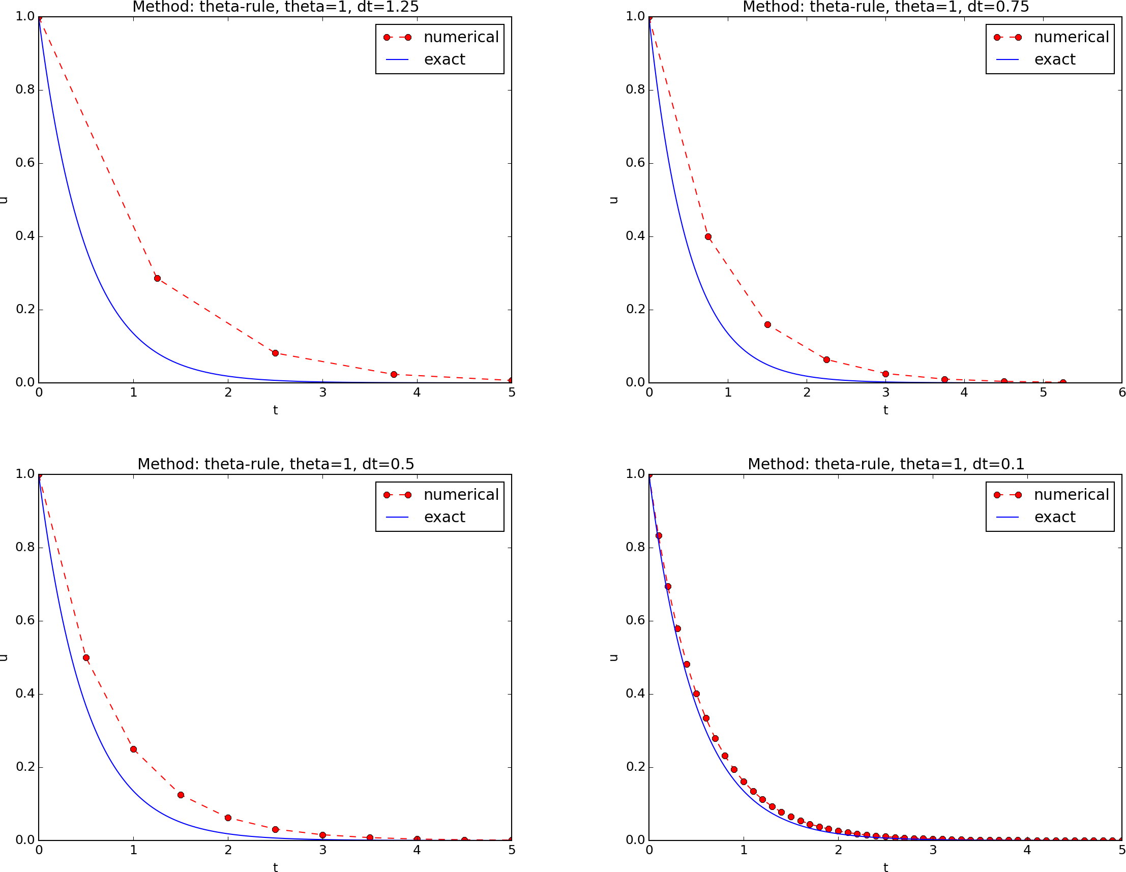
Illustration of the Backward Euler method for four time step values
The appropriate ImageMagick commands are
Terminal> montage -background white -geometry 100% -tile 2x \
          f1.png f2.png f3.png f4.png f.png
Terminal> convert -trim f.png f.png
Terminal> convert f.png -transparent white f.png
The first command mounts the four files in one, the next convert command
removes unnecessary surrounding white space, and the final convert command
makes the white background transparent.
High-quality montage of PDF files f1.pdf,
f2.pdf, f3.pdf, and f4.pdf into f.pdf goes like
Terminal> pdftk f1.pdf f2.pdf f3.pdf f4.pdf output tmp.pdf
Terminal> pdfnup --nup 2x2 --outfile tmp.pdf tmp.pdf
Terminal> pdfcrop tmp.pdf f.pdf
Terminal> rm -f tmp.pdf
Running a program from Python
The script for automating experiments needs to run the model.py program
with appropriate command-line options. Python has several tools for
executing an arbitrary command in the operating systems.
Let cmd be a string containing the desired command.
In the present case study, cmd could be 'python model.py --I 1 --dt 0.5 0.2'.
The following code
executes cmd and loads the text output into a string output:
from subprocess import Popen, PIPE, STDOUT
p = Popen(cmd, shell=True, stdout=PIPE, stderr=STDOUT)
output, _ = p.communicate()

# Check if the execution was successful
failure = p.returncode
if failure:
    print 'Command failed:', cmd; sys.exit(1)
Unsuccessful execution usually makes it meaningless to continue
the program, and therefore we abort the program with sys.exit(1).
Any argument different from 0 signifies to the computer’s operating system
that our program stopped with a failure.
Programming tip: use _ for dummy variable
Sometimes we need to unpack tuples or lists in separate variables, but we are not interested in all the variables. One example is
output, error = p.communicate()
but error is of no interest in the example above.
One can then use underscore _ as variable name for the dummy
(uninteresting) variable(s):
output, _ = p.communicate()
Here is another example where we iterate over a list of three-tuples, but the interest is limited to the second element in each three-tuple:
for _, value, _ in list_of_three_tuples:
    # work with value
We need to interpret the contents of the string
output and store
the data in an appropriate data structure for further processing.
Since the content is basically a table and will be transformed to
a spread sheet format, we let the columns in the table be represented
by lists in the program,
and we collect these columns in a dictionary whose keys are natural
column names: dt and the three values of \(\theta\).
The following code translates the output of cmd (output)
to such a dictionary of lists (errors):
errors = {'dt': dt_values, 1: [], 0: [], 0.5: []}
for line in output.splitlines():
    words = line.split()
    if words[0] in ('0.0', '0.5', '1.0'):  # line with E?
        # typical line: 0.0   1.25:    7.463E+00
        theta = float(words[0])
        E = float(words[2])
        errors[theta].append(E)
The automating script
We have now all the core elements in place to write the complete
script where we run
model.py for a set of \(\Delta t\) values (given as positional
command-line arguments), make the error plot,
write the CSV file, and combine plot files as described above.
The complete code is listed below, followed by some explaining comments.
import os, sys, glob
import matplotlib.pyplot as plt

def run_experiments(I=1, a=2, T=5):
    # The command line must contain dt values
    if len(sys.argv) > 1:
        dt_values = [float(arg) for arg in sys.argv[1:]]
    else:
        print 'Usage: %s dt1 dt2 dt3 ...' %  sys.argv[0]
        sys.exit(1)  # abort

    # Run module file and grab output
    cmd = 'python model.py --I %g --a %g --T %g' % (I, a, T)
    dt_values_str = ' '.join([str(v) for v in dt_values])
    cmd += ' --dt %s' % dt_values_str
    print cmd
    from subprocess import Popen, PIPE, STDOUT
    p = Popen(cmd, shell=True, stdout=PIPE, stderr=STDOUT)
    output, _ = p.communicate()
    failure = p.returncode
    if failure:
        print 'Command failed:', cmd; sys.exit(1)

    errors = {'dt': dt_values, 1: [], 0: [], 0.5: []}
    for line in output.splitlines():
        words = line.split()
        if words[0] in ('0.0', '0.5', '1.0'):  # line with E?
            # typical line: 0.0   1.25:    7.463E+00
            theta = float(words[0])
            E = float(words[2])
            errors[theta].append(E)

    # Find min/max for the axis
    E_min = 1E+20; E_max = -E_min
    for theta in 0, 0.5, 1:
        E_min = min(E_min, min(errors[theta]))
        E_max = max(E_max, max(errors[theta]))

    plt.loglog(errors['dt'], errors[0], 'ro-')
    plt.loglog(errors['dt'], errors[0.5], 'b+-')
    plt.loglog(errors['dt'], errors[1], 'gx-')
    plt.legend(['FE', 'CN', 'BE'], loc='upper left')
    plt.xlabel('log(time step)')
    plt.ylabel('log(error)')
    plt.axis([min(dt_values), max(dt_values), E_min, E_max])
    plt.title('Error vs time step')
    plt.savefig('error.png');  plt.savefig('error.pdf')

    # Write out a table in CSV format
    f = open('error.csv', 'w')
    f.write(r'$\Delta t$,$\theta=0$,$\theta=0.5$,$\theta=1$' + '\n')
    for _dt, _fe, _cn, _be in zip(
        errors['dt'], errors[0], errors[0.5], errors[1]):
        f.write('%.2f,%.4f,%.4f,%.4f\n' % (_dt, _fe, _cn, _be))
    f.close()

    # Combine images into rows with 2 plots in each row
    image_commands = []
    for method in 'BE', 'CN', 'FE':
        pdf_files = ' '.join(['%s_%g.pdf' % (method, dt)
                              for dt in dt_values])
        png_files = ' '.join(['%s_%g.png' % (method, dt)
                              for dt in dt_values])
        image_commands.append(
            'montage -background white -geometry 100%' +
            ' -tile 2x %s %s.png' % (png_files, method))
        image_commands.append(
            'convert -trim %s.png %s.png' % (method, method))
        image_commands.append(
            'convert %s.png -transparent white %s.png' %
            (method, method))
        image_commands.append(
            'pdftk %s output tmp.pdf' % pdf_files)
        num_rows = int(round(len(dt_values)/2.0))
        image_commands.append(
            'pdfnup --nup 2x%d --outfile tmp.pdf tmp.pdf' % num_rows)
        image_commands.append(
            'pdfcrop tmp.pdf %s.pdf' % method)

    for cmd in image_commands:
        print cmd
        failure = os.system(cmd)
        if failure:
            print 'Command failed:', cmd; sys.exit(1)

    # Remove the files generated above and by model.py
    from glob import glob
    filenames = glob('*_*.png') + glob('*_*.pdf') + glob('tmp*.pdf')
    for filename in filenames:
        os.remove(filename)

if __name__ == '__main__':
    run_experiments(I=1, a=2, T=5)
    plt.show()
We may comment upon many useful constructs in this script:
[float(arg) for arg in sys.argv[1:]]builds a list of real numbers from all the command-line arguments.['%s_%s.png' % (method, dt) for dt in dt_values]builds a list of filenames from a list of numbers (dt_values).- All
montage,convert,pdftk,pdfnup, andpdfcropcommands for creating composite figures are stored in a list and later executed in a loop.glob('*_*.png')returns a list of the names of all files in the current directory where the filename matches the Unix wildcard notation*_*.png(meaning any text, underscore, any text, and then.png).os.remove(filename)removes the file with namefilename.failure = os.system(cmd)runs an operating system command with simpler syntax than what is required bysubprocess(but the output ofcmdcannot be captured).
Making a report
The results of running computer experiments are best documented in a little report containing the problem to be solved, key code segments, and the plots from a series of experiments. At least the part of the report containing the plots should be automatically generated by the script that performs the set of experiments, because in the script we know exactly which input data that were used to generate a specific plot, thereby ensuring that each figure is connected to the right data. Take a look at a sample report to see what we have in mind.
Word, OpenOffice, GoogleDocs
Microsoft Word, its open source counterparts OpenOffice and LibreOffice, along with GoogleDocs and similar online services are the dominating tools for writing reports today. Nevertheless, scientific reports often need mathematical equations and nicely typeset computer code in monospace font. The support for mathematics and computer code in the mentioned tools is in this author’s view not on par with the technologies based on markup languages and which are addressed below. Also, with markup languages one has a readable, pure text file as source for the report, and changes in this text can easily be tracked by version control systems like Git. The result is a very strong tool for monitoring “who did what when” with the files, resulting in increased reliability of the writing process. For collaborative writing, the merge functionality in Git leads to safer simultaneously editing than what is offered even by collaborative tools like GoogleDocs.
HTML with MathJax
HTML is the markup language used for web pages. Nicely typeset computer
code is straightforward in HTML, and high-quality mathematical
typesetting is available using an extension to HTML called MathJax, which allows formulas and equations to be
typeset with LaTeX syntax and nicely rendered in web browsers, see
Figure Report in HTML format with MathJax. A relatively small
subset of LaTeX environments for mathematics is supported, but the
syntax for formulas is quite rich. Inline formulas look like \(
u'=-au \) while equations are surrounded by $$ signs. Inside such
signs, one can use \[ u'=-au \] for unnumbered equations, or
\begin{equation} and \end{equation} for
numbered equations, or \begin{equation} and \end{equation} for multiple
numbered aligned equations. You need to be familiar with mathematical
typesetting in LaTeX to write MathJax
code.
The file exper1_mathjax.py calls a script exper1.py to perform the numerical experiments and then runs Python statements for creating an HTML file with the source code for the scientific report.
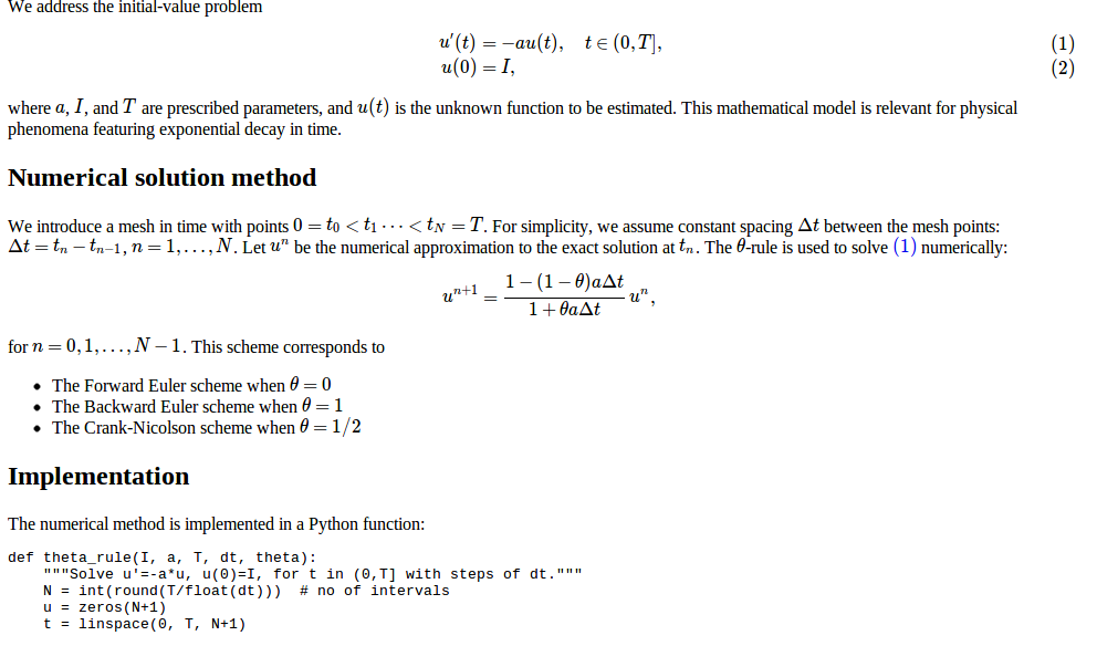
Report in HTML format with MathJax
LaTeX
The de facto language for mathematical typesetting and scientific report writing is LaTeX. A number of very sophisticated packages have been added to the language over a period of three decades, allowing very fine-tuned layout and typesetting. For output in the PDF format, see Figure Report in PDF format generated from LaTeX source for an example, LaTeX is the definite choice when it comes to typesetting quality. The LaTeX language used to write the reports has typically a lot of commands involving backslashes and braces, and many claim that LaTeX syntax is not particularly readable. For output on the web via HTML code (i.e., not only showing the PDF in the browser window), LaTeX struggles with delivering high quality typesetting. Other tools, especially Sphinx, give better results and can also produce nice-looking PDFs. The file exper1_latex.py shows how to generate the LaTeX source from a program.
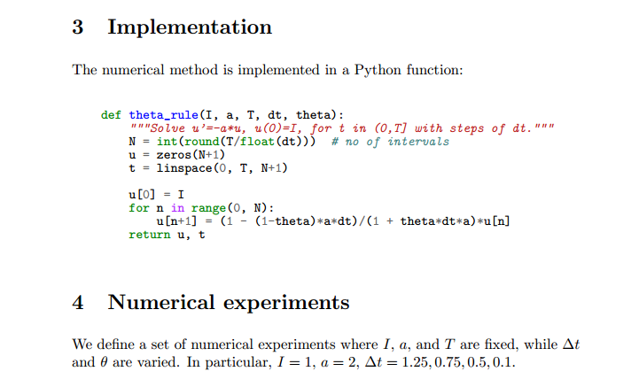
Report in PDF format generated from LaTeX source
Sphinx
Sphinx is a typesetting language with
similarities to HTML and LaTeX, but with much less tagging. It has
recently become very popular for software documentation and
mathematical reports. Sphinx can utilize LaTeX for mathematical
formulas and equations. Unfortunately, the
subset of LaTeX mathematics supported is less than in full MathJax (in
particular, numbering of multiple equations in an align type
environment is not supported). The Sphinx syntax is an extension of
the reStructuredText language. An attractive feature of Sphinx is its
rich support for fancy layout of web pages. In particular,
Sphinx can easily be combined with various layout themes that give a
certain look and feel to the web site and that offers table of
contents, navigation, and search facilities, see Figure
Report in HTML format generated from Sphinx source.
Report in HTML format generated from Sphinx source
Markdown
A recent, very popular format for easy writing of web pages is Markdown. Text is written very much like one would do in email, using spacing and special characters to naturally format the code instead of heavily tagging the text as in LaTeX and HTML. With the tool Pandoc one can go from Markdown to a variety of formats. HTML is a common output format, but LaTeX, epub, XML, OpenOffice/LibreOffice, MediaWiki, and Microsoft Word are some other possibilities. A Markdown version of our scientific report demo is available as an IPython/Jupyter notebook (described next).
IPython/Jupyter notebooks
The IPython Notebook is a web-based tool where one can write scientific reports with live computer code and graphics. Or the other way around: software can be equipped with documentation in the style of scientific reports. A slightly extended version of Markdown is used for writing text and mathematics, and the source code of a notebook is in json format. The interest in the notebook has grown amazingly fast over just a few years, and further development now takes place in the Jupyter project, which supports a lot of programming languages for interactive notebook computing. Jupyter notebooks are primarily live electronic documents, but they can be printed out as PDF reports too. A notebook version of our scientific report can be downloaded and experimented with or just statically viewed in a browser.
Wiki formats
A range of wiki formats are popular for creating notes on the web, especially documents which allow groups of people to edit and add content. Apart from MediaWiki (the wiki format used for Wikipedia), wiki formats have no support for mathematical typesetting and also limited tools for displaying computer code in nice ways. Wiki formats are therefore less suitable for scientific reports compared to the other formats mentioned here.
DocOnce
Since it is difficult to choose the right tool or format for writing a scientific report, it is advantageous to write the content in a format that easily translates to LaTeX, HTML, Sphinx, Markdown, IPython/Jupyter notebooks, and various wikis. DocOnce is such a tool. It is similar to Pandoc, but offers some special convenient features for writing about mathematics and programming. The tagging is modest, somewhere between LaTeX and Markdown. The program exper1_do.py demonstrates how to generate DocOnce code for a scientific report. There is also a corresponding rich demo of the resulting reports that can be made from this DocOnce code.
Publishing a complete project
To assist the important principle of replicable science, a report documenting scientific investigations should be accompanied by all the software and data used for the investigations so that others have a possibility to redo the work and assess the qualify of the results.
One way of documenting a complete project is to make a directory tree with all relevant files. Preferably, the tree is published at some project hosting site like Bitbucket or GitHub so that others can download it as a tarfile, zipfile, or clone the files directly using the Git version control system. For the investigations outlined in the section Making a report, we can create a directory tree with files
setup.py
./src:
   model.py
./doc:
   ./src:
      exper1_mathjax.py
      make_report.sh
      run.sh
   ./pub:
      report.html
The src directory holds source code (modules) to be reused in other projects,
the setup.py script builds and installs such software,
the doc directory contains the documentation, with src for the
source of the documentation (usually written in a markup language)
and pub for published (compiled) documentation.
The run.sh file is a simple Bash script listing the python commands
we used to run exper1_mathjax.py to generate the experiments and
the report.html file.
Exercises
Problem 5.1: Make a tool for differentiating curves
Suppose we have a curve specified through a set of discrete coordinates \((x_i,y_i)\), \(i=0,\ldots,n\), where the \(x_i\) values are uniformly distributed with spacing \(\Delta x\): \(x_i=\Delta x\). The derivative of this curve, defined as a new curve with points \((x_i, d_i)\), can be computed via finite differences:
a)
Write a function
differentiate(x, y) for differentiating a curve
with coordinates in the arrays x and y, using the
formulas above. The function should return the coordinate arrays
of the resulting differentiated curve.
b) Since the formulas for differentiation used here are only approximate, with unknown approximation errors, it is challenging to construct test cases. Here are three approaches, which should be implemented in three separate test functions.
- Consider a curve with three points and compute \(d_i\), \(i=0,1,2\), by hand. Make a test that compares the hand-calculated results with those from the function in a).
- The formulas for \(d_i\) are exact for points on a straight line, as all the \(d_i\) values are then the same, equal to the slope of the line. A test can check this property.
- For points lying on a parabola, the values for \(d_i\), \(i=1,\ldots,n-1\), should equal the exact derivative of the parabola. Make a test based on this property.
c)
Start with a curve corresponding to \(y=\sin(\pi x)\) and \(n+1\)
points in \([0,1]\). Apply differentiate four times and plot the
resulting curve and the exact \(y=\sin\pi x\) for \(n=6, 11, 21, 41\).
Filename: curvediff.
Problem 5.2: Make solid software for the Trapezoidal rule
An integral
can be numerically approximated by the Trapezoidal rule,
where \(x_i\) is a set of uniformly spaced points in \([a,b]\):
Somebody has used this rule to compute the integral \(\int_0^\pi \sin^2x\, dx\):
from math import pi, sin
np = 20
h = pi/np
I = 0
for k in range(1, np):
    I += sin(k*h)**2
print I
a) The “flat” implementation above suffers from serious flaws:
- A general numerical algorithm (the Trapezoidal rule) is implemented in a specialized form where the formula for \(f\) is inserted directly into the code for the general integration formula.
- A general numerical algorithm is not encapsulated as a general function, with appropriate parameters, which can be reused across a wide range of applications.
- The lazy programmer dropped the first terms in the general formula since \(\sin(0)=\sin(\pi)=0\).
- The sloppy programmer used
np(number of points?) as variable fornin the formula and a counterkinstead ofi. Such small deviations from the mathematical notation are completely unnecessary. The closer the code and the mathematics can get, the easier it is to spot errors in formulas.
Write a function trapezoidal that fixes these flaws.
Place the function in a module trapezoidal.
b)
Write a test function test_trapezoidal. Call the test function
explicitly to check that it works. Remove the call and run pytest
on the module:
Terminal> py.test -s -v trapezoidal
Hint. Note that even if you know the value of the integral, you do not know the error in the approximation produced by the Trapezoidal rule. However, the Trapezoidal rule will integrate linear functions exactly (i.e., to machine precision). Base a test function on a linear \(f(x)\).
c) Add functionality such that we can compute \(\int_a^b f(x)dx\) by providing \(f\), \(a\), \(b\), and \(n\) as positional command-line arguments to the module file:
Terminal> python trapezoidal.py 'sin(x)**2' 0 pi 20
Here, \(a=0\), \(b=\pi\), and \(n=20\).
Note that the trapezoidal.py file must still be a valid module file, so the
interpretation of command-line data and computation of the integral
must be performed from calls in a test block.
Hint.
To translate a string formula on the command line, like sin(x)**2,
into a Python function, you can wrap a function declaration around
the formula and run exec on the string to turn it into live Python code:
import math, sys
formula = sys.argv[1]
f_code = """
def f(x):
    return %s
""" % formula
exec(code, math.__dict__)
The result is the same as if we had hardcoded
from math import *

def f(x):
    return sin(x)**2
in the program. Note that exec needs the namespace
math.__dict__, i.e., all names in the math module, such that
it understands sin and other mathematical functions.
Similarly, to allow \(a\) and \(b\) to be math expressions like pi/4
and exp(4), do
a = eval(sys.argv[2], math.__dict__)
b = eval(sys.argv[2], math.__dict__)
d) Write a test function for verifying the implementation of data reading from the command line.
Filename: trapezoidal.
Problem 5.3: Implement classes for the Trapezoidal rule
We consider the same problem setting as in Problem 5.2: Make solid software for the Trapezoidal rule. Make a module with a class Problem
representing the mathematical problem to be solved and a class
Solver representing the solution method. The rest of the
functionality of the module, including test functions and reading data
from the command line, should be as in Problem 5.2: Make solid software for the Trapezoidal rule.
Filename: trapezoidal_class.
Problem 5.4: Write a doctest and a test function
Type in the following program:
import sys
# This sqrt(x) returns real if x>0 and complex if x<0
from numpy.lib.scimath import sqrt

def roots(a, b, c):
    """
    Return the roots of the quadratic polynomial
    p(x) = a*x**2 + b*x + c.

    The roots are real or complex objects.
    """
    q = b**2 - 4*a*c
    r1 = (-b + sqrt(q))/(2*a)
    r2 = (-b - sqrt(q))/(2*a)
    return r1, r2

a, b, c = [float(arg) for arg in sys.argv[1:]]
print roots(a, b, c)
a)
Equip the roots function with a doctest.
Make sure to test both real and complex roots.
Write out numbers in the doctest with 14 digits or less.
b)
Make a test function for the roots function. Perform the
same mathematical tests as in a), but with different
programming technology.
Filename: test_roots.
Problem 5.5: Investigate the size of tolerances in comparisons
When we replace a comparison a == b, where a and/or b are
float objects, by a comparison with tolerance, abs(a-b) < tol,
the appropriate size of tol depends on the size of a and b.
Investigate how the size of abs(a-b) varies when b takes on
values \(10^k\), \(k=-5,-9,\ldots,20\) and a=1.0/49*b*49.
Thereafter, compute the relative difference abs((a-b)/a) for
the same b values.
Filename: tolerance.
Remarks
You will experience that if a and b are large, as they can be
in, e.g.,
geophysical applications where lengths measured in meters can be of size
\(10^6\) m, tol must be about \(10^{-9}\), while a and b around unity can
have tol of size \(10^{-15}\).
The way out of the problem with choosing a tolerance is to use
relative differences.
Exercise 5.6: Make use of a class implementation
Implement the experiment_compare_dt function from decay.py
using class Problem and class Solver from
the section Classes for problem and solution method.
The parameters I, a, T, the scheme name, and a series of
dt values should be read from the command line.
Filename: experiment_compare_dt_class.
Problem 5.7: Make solid software for a difference equation
We have the following evolutionary difference equation for the number of individuals \(u^n\) of a certain specie at time \(n\Delta t\):
Here, \(n\) is a counter in time, \(\Delta t\) is time between time levels
\(n\) and \(n+1\) (assumed constant), \(r\) is a net reproduction rate
for the specie,
and \(M^n\) is the upper limit of the population that the environment can
sustain at time level \(n\).
Filename: logistic.
