Models
This chapter presents many mathematical models that all end up with ODEs of the type \(u^{\prime}=-au+b\). The applications are taken from biology, finance, and physics, and cover population growth or decay, interacting predator-prey populations, compound interest and inflation, radioactive decay, chemical and biochemical reaction, spreading of diseases, cooling of objects, compaction of geological media, pressure variations in the atmosphere, viscoelastic response in materials, and air resistance on falling or rising bodies.
Before we turn to the applications, however, we take a brief look at the technique of scaling, which is so useful in many applications.
Scaling
Real applications of a model \(u^{\prime}=-au+b\) will often involve a lot of parameters in the expressions for \(a\) and \(b\). It can be quite a challenge to find relevant values of all parameters. In simple problems, however, it turns out that it is not always necessary to estimate all parameters because we can lump them into one or a few dimensionless numbers by using a very attractive technique called scaling. It simply means to stretch the \(u\) and \(t\) axis in the present problem - and suddenly all parameters in the problem are lumped into one parameter if \(b\neq 0\) and no parameter when \(b=0\)!
Dimensionless variables
Scaling means that we introduce a new function \(\bar u(\bar t)\), with
where \(u_m\) is a characteristic value of \(u\), \(u_c\) is a characteristic size of the range of \(u\) values, and \(t_c\) is a characteristic size of the range of \(t\) where \(u\) shows significant variation. Choosing \(u_m\), \(u_c\), and \(t_c\) is not always easy and is often an art in complicated problems. We just state one choice first:
Inserting \(u=u_m + u_c\bar u\) and \(t=t_c\bar t\) in the problem \(u^{\prime}=-au + b\), assuming \(a\) and \(b\) are constants, results (after some algebra) in the scaled problem
where
Dimensionless numbers
The parameter \(\beta\) is a dimensionless number. From the equation we see that \(b\) must have the same unit as the term \(au\). The initial condition \(I\) must have the same unit as \(u\), so \(Ia\) has the same unit as \(b\), making the fraction \(b/(Ia)\) dimensionless.
An important observation is that \(\bar u\) depends on \(\bar t\) and \(\beta\). That is, only the special combination of \(b/(Ia)\) matters, not what the individual values of \(b\), \(a\), and \(I\) are. The original unscaled function \(u\) depends on \(t\), \(b\), \(a\), and \(I\).
A second observation is striking: if \(b=0\), the scaled problem is independent of \(a\) and \(I\)! In practice this means that we can perform a single numerical simulation of the scaled problem and recover the solution of any problem for a given \(a\) and \(I\) by stretching the axis in the plot: \(u=I\bar u\) and \(t =\bar t/a\). For \(b\neq 0\), we simulate the scaled problem for a few \(\beta\) values and recover the physical solution \(u\) by translating and stretching the \(u\) axis and stretching the \(t\) axis.
In general, scaling combines the parameters in a problem to a set of dimensionless parameters. The number of dimensionless parameters is usually much smaller than the number of original parameters. The section Vertical motion of a body in a viscous fluid presents an example where 11 parameters are reduced to one!
A scaling for vanishing initial condition
The scaling breaks down if \(I=0\). In that case we may choose \(u_m=0\), \(u_c=b/a\), and \(t_c=1/b\), resulting in a slightly different scaled problem:
As with \(b=0\), the case \(I=0\) has a scaled problem with no physical parameters!
It is common to drop the bars after scaling and write the scaled problem as \(u^{\prime}=-u\), \(u(0)=1-\beta\), or \(u^{\prime}=1-u\), \(u(0)=0\). Any implementation of the problem \(u^{\prime}=-au+b\), \(u(0)=I\), can be reused for the scaled problem by setting \(a=1\), \(b=0\), and \(I=1-\beta\) in the code, if \(I\neq 0\), or one sets \(a=1\), \(b=1\), and \(I=0\) when the physical \(I\) is zero. Falling bodies in fluids, as described in the section Vertical motion of a body in a viscous fluid, involves \(u^{\prime}=-au+b\) with seven physical parameters. All these vanish in the scaled version of the problem if we start the motion from rest!
Many more details about scaling are presented in the author’s book Scaling of Differential Equations [Ref11].
Evolution of a population
Exponential growth
Let \(N\) be the number of individuals in a population occupying some spatial domain. Despite \(N\) being an integer in this problem, we shall compute with \(N\) as a real number and view \(N(t)\) as a continuous function of time. The basic model assumption is that in a time interval \(\Delta t\) the number of newcomers to the populations (newborns) is proportional to \(N\), with proportionality constant \(\bar b\). The amount of newcomers will increase the population and result in
It is obvious that a long time interval \(\Delta t\) will result in more newcomers and hence a larger \(\bar b\). Therefore, we introduce \(b=\bar b/\Delta t\): the number of newcomers per unit time and per individual. We must then multiply \(b\) by the length of the time interval considered and by the population size to get the total number of new individuals, \(b\Delta t N\).
If the number of removals from the population (deaths) is also proportional to \(N\), with proportionality constant \(d\Delta t\), the population evolves according to
Dividing by \(\Delta t\) and letting \(\Delta t \rightarrow 0\), we get the ODE
In a population where the death rate (\(d\)) is larger than then newborn rate (\(b\)), \(b-d < 0\), and the population experiences exponential decay rather than exponential growth.
In some populations there is an immigration of individuals into the spatial domain. With \(I\) individuals coming in per time unit, the equation for the population change becomes
The corresponding ODE reads
Emigration is also modeled by this \(I\) term if we just change its sign: \(I < 0\). So, the \(I\) term models migration in and out of the domain in general.
Some simplification arises if we introduce a fractional measure of the population: \(u=N/N_0\) and set \(r=b-d\). The ODE problem now becomes
where \(f=I/N_0\) measures the net immigration per time unit as the fraction of the initial population. Very often, \(r\) is approximately constant, but \(f\) is usually a function of time.
Logistic growth
The growth rate \(r\) of a population decreases if the environment has limited resources. Suppose the environment can sustain at most \(N_{\max}\) individuals. We may then assume that the growth rate approaches zero as \(N\) approaches \(N_{\max}\), i.e., as \(u\) approaches \(M=N_{\max}/N_0\). The simplest possible evolution of \(r\) is then a linear function: \(r(t)={\varrho}(1-u(t)/M)\), where \(\varrho\) is the initial growth rate when the population is small relative to the maximum size and there is enough resources. Using this \(r(t)\) in (129) results in the logistic model for the evolution of a population (assuming for the moment that \(f=0\)):
Initially, \(u\) will grow at rate \(\varrho\), but the growth will decay as \(u\) approaches \(M\), and then there is no more change in \(u\), causing \(u\rightarrow M\) as \(t\rightarrow\infty\). Note that the logistic equation \(u^{\prime}={\varrho}(1-u/M)u\) is nonlinear because of the quadratic term \(-u^2{\varrho}/M\).
Compound interest and inflation
Say the annual interest rate is \(r\) percent and that the bank adds the interest once a year to your investment. If \(u^n\) is the investment in year \(n\), the investment in year \(u^{n+1}\) grows to
In reality, the interest rate is added every day. We therefore introduce a parameter \(m\) for the number of periods per year when the interest is added. If \(n\) counts the periods, we have the fundamental model for compound interest:
This model is a difference equation, but it can be transformed to a continuous differential equation through a limit process. The first step is to derive a formula for the growth of the investment over a time \(t\). Starting with an investment \(u^0\), and assuming that \(r\) is constant in time, we get
Introducing time \(t\), which here is a real-numbered counter for years, we have that \(n=mt\), so we can write
The second step is to assume continuous compounding, meaning that the interest is added continuously. This implies \(m\rightarrow\infty\), and in the limit one gets the formula
which is nothing but the solution of the ODE problem
This is then taken as the ODE model for compound interest if \(r>0\). However, the reasoning applies equally well to inflation, which is just the case \(r < 0\). One may also take the \(r\) in (133) as the net growth of an investment, where \(r\) takes both compound interest and inflation into account. Note that for real applications we must use a time-dependent \(r\) in (133).
Introducing \(a=\frac{r}{100}\), continuous inflation of an initial fortune \(I\) is then a process exhibiting exponential decay according to
Newton’s law of cooling
When a body at some temperature is placed in a cooling environment, experience shows that the temperature falls rapidly in the beginning, and then the change in temperature levels off until the body’s temperature equals that of the surroundings. Newton carried out some experiments on cooling hot iron and found that the temperature evolved as a “geometric progression at times in arithmetic progression”, meaning that the temperature decayed exponentially. Later, this result was formulated as a differential equation: the rate of change of the temperature in a body is proportional to the temperature difference between the body and its surroundings. This statement is known as Newton’s law of cooling, which mathematically can be expressed as
where \(T\) is the temperature of the body, \(T_s\) is the temperature of the surroundings (which may be time-dependent), \(t\) is time, and \(k\) is a positive constant. Equation (134) is primarily viewed as an empirical law, valid when heat is efficiently convected away from the surface of the body by a flowing fluid such as air at constant temperature \(T_s\). The heat transfer coefficient \(k\) reflects the transfer of heat from the body to the surroundings and must be determined from physical experiments.
The cooling law (134) needs an initial condition \(T(0)=T_0\).
Radioactive decay
An atomic nucleus of an unstable atom may lose energy by emitting ionizing particles and thereby be transformed to a nucleus with a different number of protons and neutrons. This process is known as radioactive decay. Actually, the process is stochastic when viewed for a single atom, because it is impossible to predict exactly when a particular atom emits a particle. Nevertheless, with a large number of atoms, \(N\), one may view the process as deterministic and compute the mean behavior of the decay. Below we reason intuitively about an ODE for the mean behavior. Thereafter, we show mathematically that a detailed stochastic model for single atoms leads to the same mean behavior.
Deterministic model
Suppose at time \(t\), the number of the original atom type is \(N(t)\). A basic model assumption is that the transformation of the atoms of the original type in a small time interval \(\Delta t\) is proportional to \(N\), so that
where \(a>0\) is a constant. The proportionality factor is \(a\Delta t\), i.e., proportional to \(\Delta t\) since a longer time interval will produce more transformations. We can introduce \(u=N(t)/N(0)\), divide by \(\Delta t\), and let \(\Delta t\rightarrow 0\):
The left-hand side is the derivative of \(u\). Dividing by the \(N_0\) gives the following ODE for \(u\):
The parameter \(a\) can for a given nucleus be expressed through the half-life \(t_{1/2}\), which is the time taken for the decay to reduce the initial amount by one half, i.e., \(u(t_{1/2}) = 0.5\). With \(u(t)=e^{-at}\), we get \(t_{1/2}=a^{-1}\ln 2\) or \(a=\ln 2/t_{1/2}\).
Stochastic model
Originally, we have \(N_0\) atoms. Up to some particular time \(t\), each atom may either have decayed or not. If not, they have “survived”. We want to count how many original atoms that have survived. The survival of a single atom at time \(t\) is a random event. Since there are only two outcomes, survival or decay, we have a Bernoulli trial. Let \(p\) be the probability of survival (implying that the probability of decay is \(1-p\)). If each atom survives independently of the others, and the probability of survival is the same for every atom, we have \(N_0\) Bernoulli trials, known as a binomial experiment from probability theory. The probability \(P(N)\) that \(N\) out of the \(N_0\) atoms have survived at time \(t\) is then given by the famous binomial distribution
The mean (or expected) value \({\hbox{E}\lbrack P \rbrack}\) of \(P(N)\) is known to be \(N_0p\).
It remains to estimate \(p\). Let the interval \([0,t]\) be divided into \(m\) small subintervals of length \(\Delta t\). We make the assumption that the probability of decay of a single atom in an interval of length \(\Delta t\) is \(\tilde p\), and that this probability is proportional to \(\Delta t\): \(\tilde p = \lambda\Delta t\) (it sounds natural that the probability of decay increases with \(\Delta t\)). The corresponding probability of survival is \(1-\lambda\Delta t\). Believing that \(\lambda\) is independent of time, we have, for each interval of length \(\Delta t\), a Bernoulli trial: the atom either survives or decays in that interval. Now, \(p\) should be the probability that the atom survives in all the intervals, i.e., that we have \(m\) successful Bernoulli trials in a row and therefore
The expected number of atoms of the original type at time \(t\) is
To see the relation between the two types of Bernoulli trials and the ODE above, we go to the limit \(\Delta t\rightarrow 0\), \(m\rightarrow\infty\). It is possible to show that
This is the famous exponential waiting time (or arrival time) distribution for a Poisson process in probability theory (obtained here, as often done, as the limit of a binomial experiment). The probability of decay, or more precisely that at least one atom has undergone a transition, is \(1-p= 1-e^{-\lambda t}\). This is the exponential distribution. The limit means that \(m\) is very large, hence \(\Delta t\) is very small, and \(\tilde p=\lambda\Delta t\) is very small since the intensity of the events, \(\lambda\), is assumed finite. This situation corresponds to a very small probability that an atom will decay in a very short time interval, which is a reasonable model. The same model occurs in lots of different applications, e.g., when waiting for a taxi, or when finding defects along a rope.
Relation between stochastic and deterministic models
With \(p=e^{-\lambda t}\) we get the expected number of original atoms at \(t\) as \(N_0p=N_0e^{-\lambda t}\), which is exactly the solution of the ODE model \(N^{\prime}=-\lambda N\). This also gives an interpretation of \(a\) via \(\lambda\) or vice versa. Our important finding here is that the ODE model captures the mean behavior of the underlying stochastic model. This is, however, not always the common relation between microscopic stochastic models and macroscopic “averaged” models.
Also of interest, is that a Forward Euler discretization of \(N^{\prime}=-\lambda N\), \(N(0)=N_0\), gives \(N^m = N_0(1-\lambda\Delta t)^m\) at time \(t_m=m\Delta t\), which is exactly the expected value of the stochastic experiment with \(N_0\) atoms and \(m\) small intervals of length \(\Delta t\), where each atom can decay with probability \(\lambda\Delta t\) in an interval.
A fundamental question is how accurate the ODE model is. The underlying stochastic model fluctuates around its expected value. A measure of the fluctuations is the standard deviation of the binomial experiment with \(N_0\) atoms, which can be shown to be \({\hbox{Std}\lbrack P \rbrack}=\sqrt{N_0p(1-p)}\). Compared to the size of the expectation, we get the normalized standard deviation
showing that the normalized fluctuations are very small if \(N_0\) is very large, which is usually the case.
Generalization of the radioactive decay modeling
The modeling in the section Radioactive decay is in fact very general, despite a focus on a particular physical process. We may instead of atoms and decay speak about a set of items, where each item can undergo a stochastic transition from one state to another. In the section Chemical kinetics the item is a molecule and the transition is a chemical reaction, while in the section Spreading of diseases the item is an ill person and the transition is recovering from the illness (or an immune person who loses her immunity).
From the modeling in the section Radioactive decay we can establish a deterministic model for a large number of items and a stochastic model for an arbitrary number of items, even a single one. The stochastic model has a parameter \(\lambda\) reflecting the probability that a transition takes place in a time interval of unit length (or equivalently, that the probability is \(\lambda\Delta t\) for a transition during a time interval of length \(\Delta t\)). The probability of making a transition before time \(t\) is given by
The corresponding probability density is \(f(t)=F'(t)=e^{-\lambda t}\). The expected value of \(F(t)\), i.e., the expected time to transition, is \(\lambda^{-1}\). This interpretation of \(\lambda\) makes it easy to measure its value: just carry out a large number of experiments, measure the time to transition, and take one over the average of these times as an estimate of \(\lambda\). The variance is \(\lambda^{-2}\).
The deterministic model counts how many items, \(N(t)\), that have undergone the transition (on average), and \(N(t)\) is governed by the ODE
Chemical kinetics
Irreversible reaction of two substances
Consider two chemical substances, A and B, and a chemical reaction that turns A into B. In a small time interval, some of the molecules of type A are transformed into molecules of B. This process is, from a mathematical modeling point of view, equivalent to the radioactive decay process described in the previous section. We can therefore apply the same modeling approach. If \(N_A\) is the number of molecules of substance A, we have that \(N_A\) is governed by the differential equation
where (the constant) \(k\) is called the rate constant of the reaction. Rather than using the number of molecules, we use the concentration of molecules: \([A](t) = N_A(t)/N_A(0)\). We see that \(d[A]/dt = N_A(0)^{-1} dN_A/dt\). Replacing \(N_A\) by \([A]\) in the equation for \(N_A\) leads to the equation for the concentration \([A]\):
Since substance A is transformed to substance B, we have that the concentration of \([B]\) grows by the loss of \([A]\):
The mathematical model can either be (137) or the system
This reaction is known as a first-order reaction, where each molecule of A makes an independent decision about whether to complete the reaction, i.e., independent of what happens to any other molecule.
An \(n\)-th order reaction is modeled by
for \(t\in (0,T]\) with initial conditions \([A](0) = 1\) and \([B](0) = 0\). Here, \(n\) can be a real number, but is most often an integer. Note that the sum of the concentrations is constant since
Reversible reaction of two substances
Let the chemical reaction turn substance A into B and substance B into A. The rate of change of \([A]\) has then two contributions: a loss \(k_A[A]\) and a gain \(k_B[B]\):
Similarly for substance B,
This time we have allowed for arbitrary initial concentrations. Again,
Irreversible reaction of two substances into a third
Now we consider two chemical substances, A and B, reacting with each other and producing a substance C. In a small time interval \(\Delta t\), molecules of type A and B are occasionally colliding, and in some of the collisions, a chemical reaction occurs, which turns A and B into a molecule of type C. (More generally, \(M_A\) molecules of A and \(M_B\) molecules of B react to form \(M_C\) molecules of \(C\).) The number of possible pairings, and thereby collisions, of A and B is \(N_AN_B\), where \(N_A\) is the number of molecules of A, and \(N_B\) is the number of molecules of B. A fraction \(k\) of these collisions, \(\hat k\Delta t N_AN_B\), features a chemical reaction and produce \(N_C\) molecules of C. The fraction is thought to be proportional to \(\Delta t\): considering a twice as long time interval, twice as many molecules collide, and twice as many reactions occur. The increase in molecules of substance C is now found from the reasoning
Dividing by \(\Delta t\),
and letting \(\Delta t\rightarrow 0\), gives the differential equation
(This equation is known as the important law of mass action discovered by the Norwegian scientists Cato M. Guldberg and Peter Waage. A more general form of the right-hand side is \(\hat kN_A^{\alpha}N_B^{\beta}\). All the constants \(\hat k\), \(\alpha\), and \(\beta\) must be determined from experiments.)
Working instead with concentrations, we introduce \([C](t)=N_C(t)/N_C(0)\), with similar definitions for \([A]\) and \([B]\) we get
The constant \(k\) is related to \(\hat k\) by \(k = \hat k N_A(0)N_B(0)/N_C(0)\). The gain in C is a loss of A and B:
A biochemical reaction
A common reaction (known as Michaelis-Menton kinetics) turns a substrate S into a product P with aid of an enzyme E. The reaction is a two-stage process: first S and E reacts to form a complex ES, where the enzyme and substrate are bound to each other, and then ES is turned into E and P. In the first stage, S and E react to produce a growth of ES according to the law of mass action:
The complex ES reacts and produces the product \(P\) at rate \(-k_{v}[ES]\) and E at rate \(-k_-[ES]\). The total set of reactions can then be expressed by
The initial conditions are \([ES](0)=[P](0)=0\), and \([S]=S_0\), \([E]=E_0\). The constants \(k_+\), \(k_-\), and \(k_v\) must be determined from experiments.
Spreading of diseases
The modeling of spreading of diseases is very similar to the modeling of chemical reactions in the section Chemical kinetics. The field of epidemiology speaks about susceptibles: people who can get a disease; infectives: people who are infected and can infect susceptibles; and recovered: people who have recovered from the disease and become immune. Three categories are accordingly defined: S for susceptibles, I for infectives, and R for recovered. The number in each category is tracked by the functions \(S(t)\), \(I(t)\), and \(R(t)\).
To model how many people that get infected in a small time interval \(\Delta t\), we reason as with reactions in the section Chemical kinetics. The possible number of pairings (“collisions”) between susceptibles and infected is \(SI\). A fraction of these, \(\beta\Delta t SI\), will actually meet and the infected succeed in infecting the susceptible, where \(\beta\) is a parameter to be empirically estimated. This leads to a loss of susceptibles and a gain of infected:
In the same time interval, a fraction \(\nu\Delta t I\) of the infected is recovered. It follows from the section Generalization of the radioactive decay modeling that the parameter \(\nu^{-1}\) is interpreted as the average waiting time to leave the I category, i.e., the average length of the disease. The \(\nu \Delta tI\) term is a loss for the I category, but a gain for the R category:
Dividing these equations by \(\Delta t\) and going to the limit \(\Delta t\rightarrow 0\), gives the ODE system
with initial values \(S(0)=S_0\), \(I(0)=I_0\), and \(R(0)=0\). By adding the equations, we realize that
where \(N\) is the total number in the population under consideration. This property can be used as a partial verification during simulations.
Equations (153)-(155) are known as the SIR model in epidemiology. The model can easily be extended to incorporate vaccination programs, immunity loss after some time, etc. Typical diseases that can be simulated by the SIR model and its variants are measles, smallpox, flu, plague, and HIV.
Predator-prey models in ecology
A model for the interaction of predator and prey species can be based on reasoning from population dynamics and the SIR model. Let \(H(t)\) be the number of preys in a region, and let \(L(t)\) be the number of predators. For example, \(H\) may be hares and \(L\) lynx, or rabbits and foxes.
The population of the prey evolves due to births and deaths, exactly as in a population dynamics model from the section Exponential growth. During a time interval \(\Delta t\) the increase in the population is therefore
where \(a\) is a parameter to be measured from data. The increase is proportional to \(H\), and the proportionality constant \(a\Delta t\) is proportional to \(\Delta t\), because doubling the interval will double the increase.
However, the prey population has an additional loss because they are eaten by predators. All the prey and predator animals can form \(LH\) pairs in total (assuming all individuals meet randomly). A small fraction \(b\Delta t\) of such meetings, during a time interval \(\Delta t\), ends up with the predator eating the prey. The increase in the prey population is therefore adjusted to
The predator population increases as a result of eating preys. The amount of eaten preys is \(b\Delta t LH\), but only a fraction \(d\Delta t LH\) of this amount contributes to increasing the predator population. In addition, predators die and this loss is set to \(c\Delta t L\). To summarize, the increase in the predator population is given by
Dividing by \(\Delta t\) in the equations for \(H\) and \(L\) and letting \(t\rightarrow 0\) results in
We can simplify the notation to the following two ODEs:
This is a so-called Lokta-Volterra model. It contains four parameters that must be estimated from data: \(a\), \(b\), \(c\), and \(d\). In addition, two initial conditions are needed for \(H(0)\) and \(L(0)\).
Decay of atmospheric pressure with altitude
The general model
Vertical equilibrium of air in the atmosphere is governed by the equation
Here, \(p(z)\) is the air pressure, \(\varrho\) is the density of air, and \(g=9.807\hbox{ m/s}^2\) is a standard value of the acceleration of gravity. (Equation (158) follows directly from the general Navier-Stokes equations for fluid motion, with the assumption that the air does not move.)
The pressure is related to density and temperature through the ideal gas law
where \(M\) is the molar mass of the Earth’s air (0.029 kg/mol), \(R^*\) is the universal gas constant (\(8.314\) Nm/(mol K)), and \(T\) is the temperature in Kelvin. All variables \(p\), \(\varrho\), and \(T\) vary with the height \(z\). Inserting (159) in (158) results in an ODE with a variable coefficient:
Multiple atmospheric layers
The atmosphere can be approximately modeled by seven layers. In each layer, (160) is applied with a linear temperature of the form
where \(z=h_i\) denotes the bottom of layer number \(i\), having temperature \(\bar T_i\), and \(L_i\) is a constant in layer number \(i\). The table below lists \(h_i\) (m), \(\bar T_i\) (K), and \(L_i\) (K/m) for the layers \(i=0,\ldots,6\).
| \(i\) | \(h_i\) | \(\bar T_i\) | \(L_i\) |
|---|---|---|---|
| 0 | 0 | 288 | -0.0065 |
| 1 | 11,000 | 216 | 0.0 |
| 2 | 20,000 | 216 | 0.001 |
| 3 | 32,000 | 228 | 0.0028 |
| 4 | 47,000 | 270 | 0.0 |
| 5 | 51,000 | 270 | -0.0028 |
| 6 | 71,000 | 214 | -0.002 |
For implementation it might be convenient to write (160) on the form
where \(\bar T(z)\), \(L(z)\), and \(h(z)\) are piecewise constant functions with values given in the table. The value of the pressure at the sea level \(z=0\), \(p_0=p(0)\), is \(101325\) Pa.
Simplifications
Constant layer temperature
One common simplification is to assume that the temperature is constant within each layer. This means that \(L=0\).
One-layer model
Another commonly used approximation is to work with one layer instead of seven. This one-layer model is based on \(T(z)=T_0 - Lz\), with sea level standard temperature \(T_0=288\) K and temperature lapse rate \(L=0.0065\) K/m.
Compaction of sediments
Sediments, originally made from materials like sand and mud, get compacted through geological time by the weight of new material that is deposited on the sea bottom. The porosity \(\phi\) of the sediments tells how much void (fluid) space there is between the sand and mud grains. The porosity drops with depth, due to the weight of the sediments above. This makes the void space shrink, and thereby compaction increases.
A typical assumption is that the change in \(\phi\) at some depth \(z\) is negatively proportional to \(\phi\). This assumption leads to the differential equation problem
where the \(z\) axis points downwards, \(z=0\) is the surface with known porosity, and \(c>0\) is a constant.
The upper part of the Earth’s crust consists of many geological layers stacked on top of each other, as indicated in Figure Illustration of the compaction of geological layers (with different colors) through time. The model (162) can be applied for each layer. In layer number \(i\), we have the unknown porosity function \(\phi_i(z)\) fulfilling \(\phi_i^{\prime}(z)=-c_iz\), since the constant \(c\) in the model (162) depends on the type of sediment in the layer. Alternatively, we can use (162) to describe the porosity through all layers if \(c\) is taken as a piecewise constant function of \(z\), equal to \(c_i\) in layer \(i\). From the figure we see that new layers of sediments are deposited on top of older ones as time progresses. The compaction, as measured by \(\phi\), is rapid in the beginning and then decreases (exponentially) with depth in each layer.
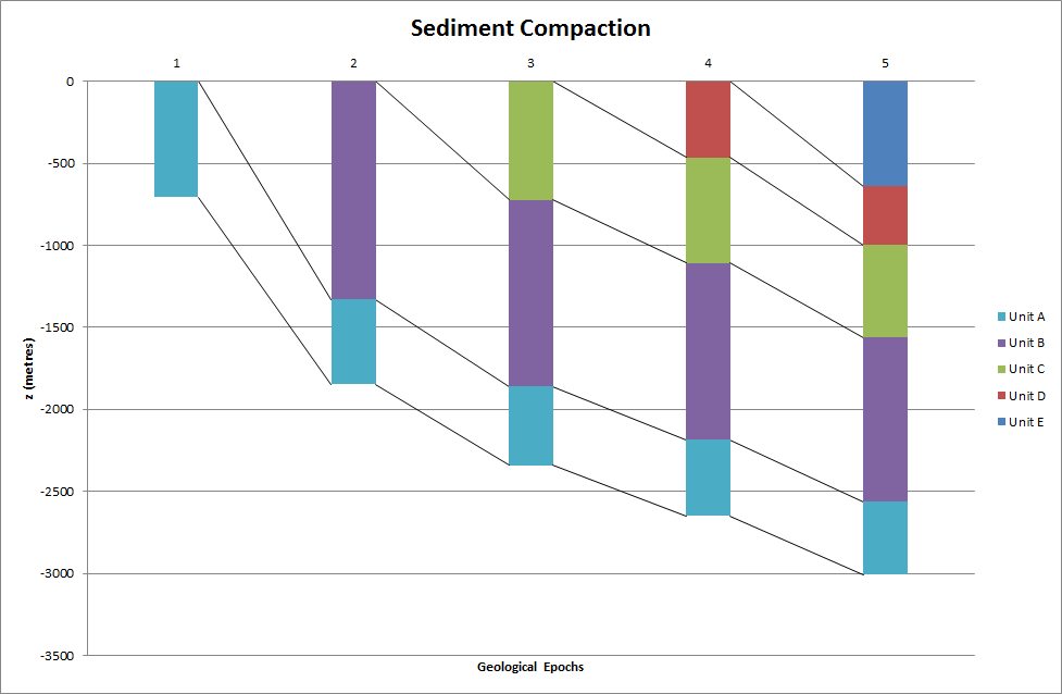
Illustration of the compaction of geological layers (with different colors) through time
When we drill a well at present time through the right-most column of sediments in Figure Illustration of the compaction of geological layers (with different colors) through time, we can measure the thickness of the sediment in (say) the bottom layer. Let \(L_1\) be this thickness. Assuming that the volume of sediment remains constant through time, we have that the initial volume, \(\int_0^{L_{1,0}} \phi_1 dz\), must equal the volume seen today, \(\int_{\ell-L_1}^{\ell}\phi_1 dz\), where \(\ell\) is the depth of the bottom of the sediment in the present day configuration. After having solved for \(\phi_1\) as a function of \(z\), we can then find the original thickness \(L_{1,0}\) of the sediment from the equation
In hydrocarbon exploration it is important to know \(L_{1,0}\) and the compaction history of the various layers of sediments.
Vertical motion of a body in a viscous fluid
A body moving vertically through a fluid (liquid or gas) is subject to three different types of forces: the gravity force, the drag force, and the buoyancy force.
Overview of forces
Taking the upward direction as positive, the gravity force is \(F_g= -mg\), where \(m\) is the mass of the body and \(g\) is the acceleration of gravity. The uplift or buoyancy force (“Archimedes force”) is \(F_b = \varrho gV\), where \(\varrho\) is the density of the fluid and \(V\) is the volume of the body.
The drag force is of two types, depending on the Reynolds number
where \(d\) is the diameter of the body in the direction perpendicular to the flow, \(v\) is the velocity of the body, and \(\mu\) is the dynamic viscosity of the fluid. When \(\hbox{Re} < 1\), the drag force is fairly well modeled by the so-called Stokes’ drag, which for a spherical body of diameter \(d\) reads
Quantities are taken as positive in the upwards vertical direction, so if \(v>0\) and the body moves upwards, the drag force acts downwards and become negative, in accordance with the minus sign in expression for \(F_d^{(S)}\).
For large Re, typically \(\hbox{Re} > 10^3\), the drag force is quadratic in the velocity:
where \(C_D\) is a dimensionless drag coefficient depending on the body’s shape, and \(A\) is the cross-sectional area as produced by a cut plane, perpendicular to the motion, through the thickest part of the body. The superscripts \(\,{}^q\) and \(\,{}^S\) in \(F_d^{(S)}\) and \(F_d^{(q)}\) indicate Stokes drag and quadratic drag, respectively.
Equation of motion
All the mentioned forces act in the vertical direction. Newton’s second law of motion applied to the body says that the sum of these forces must equal the mass of the body times its acceleration \(a\) in the vertical direction.
Here we have chosen to model the fluid resistance by the Stokes drag. Inserting the expressions for the forces yields
The unknowns here are \(v\) and \(a\), i.e., we have two unknowns but only one equation. From kinematics in physics we know that the acceleration is the time derivative of the velocity: \(a = dv/dt\). This is our second equation. We can easily eliminate \(a\) and get a single differential equation for \(v\):
A small rewrite of this equation is handy: We express \(m\) as \(\varrho_bV\), where \(\varrho_b\) is the density of the body, and we divide by the mass to get
We may introduce the constants
so that the structure of the differential equation becomes obvious:
The corresponding initial condition is \(v(0)=v_0\) for some prescribed starting velocity \(v_0\).
This derivation can be repeated with the quadratic drag force \(F_d^{(q)}\), leading to the result
Defining
and \(b\) as above, we can write (169) as
Terminal velocity
An interesting aspect of (168) and (171) is whether \(v\) will approach a final constant value, the so-called terminal velocity \(v_T\), as \(t\rightarrow\infty\). A constant \(v\) means that \(v^{\prime}(t)\rightarrow 0\) as \(t\rightarrow\infty\) and therefore the terminal velocity \(v_T\) solves
and
The former equation implies \(v_T = b/a\), while the latter has solutions \(v_T =-\sqrt{|b|/a}\) for a falling body (\(v_T < 0\)) and \(v_T = \sqrt{b/a}\) for a rising body (\(v_T>0\)).
A Crank-Nicolson scheme
Both governing equations, the Stokes’ drag model (168) and the quadratic drag model (171), can be readily solved by the Forward Euler scheme. For higher accuracy one can use the Crank-Nicolson method, but a straightforward application of this method gives a nonlinear equation in the new unknown value \(v^{n+1}\) when applied to (171):
The first term on the right-hand side of (172) is the arithmetic average of \(-|v|v\) evaluated at time levels \(n\) and \(n+1\).
Instead of approximating the term \(-|v|v\) by an arithmetic average, we can use a geometric mean:
The error is of second order in \(\Delta t\), just as for the arithmetic average and the centered finite difference approximation in (172). With the geometric mean, the resulting discrete equation
becomes a linear equation in \(v^{n+1}\), and we can therefore easily solve for \(v^{n+1}\):
Using a geometric mean instead of an arithmetic mean in the Crank-Nicolson scheme is an attractive method for avoiding a nonlinear algebraic equation when discretizing a nonlinear ODE.
Physical data
Suitable values of \(\mu\) are \(1.8\cdot 10^{-5}\hbox{ Pa}\, \hbox{s}\) for air and \(8.9\cdot 10^{-4}\hbox{ Pa}\, \hbox{s}\) for water. Densities can be taken as \(1.2\hbox{ kg/m}^3\) for air and as \(1.0\cdot 10^3\hbox{ kg/m}^3\) for water. For considerable vertical displacement in the atmosphere one should take into account that the density of air varies with the altitude, see the section Decay of atmospheric pressure with altitude. One possible density variation arises from the one-layer model in the mentioned section.
Any density variation makes \(b\) time dependent and we need \(b^{n+\frac{1}{2}}\) in (174). To compute the density that enters \(b^{n+\frac{1}{2}}\) we must also compute the vertical position \(z(t)\) of the body. Since \(v=dz/dt\), we can use a centered difference approximation:
This \(z^{n+\frac{1}{2}}\) is used in the expression for \(b\) to compute \(\varrho(z^{n+\frac{1}{2}})\) and then \(b^{n+\frac{1}{2}}\).
The drag coefficient \(C_D\) depends heavily on the shape of the body. Some values are: 0.45 for a sphere, 0.42 for a semi-sphere, 1.05 for a cube, 0.82 for a long cylinder (when the center axis is in the vertical direction), 0.75 for a rocket, 1.0-1.3 for a man in upright position, 1.3 for a flat plate perpendicular to the flow, and 0.04 for a streamlined, droplet-like body.
Verification
To verify the program, one may assume a heavy body in air such that the \(F_b\) force can be neglected, and further assume a small velocity such that the air resistance \(F_d\) can also be neglected. This can be obtained by setting \(\mu\) and \(\varrho\) to zero. The motion then leads to the velocity \(v(t)=v_0 - gt\), which is linear in \(t\) and therefore should be reproduced to machine precision (say tolerance \(10^{-15}\)) by any implementation based on the Crank-Nicolson or Forward Euler schemes.
Another verification, but not as powerful as the one above, can be based on computing the terminal velocity and comparing with the exact expressions. The advantage of this verification is that we can also test the situation \(\varrho\neq 0\).
As always, the method of manufactured solutions can be applied to test the implementation of all terms in the governing equation, but then the solution has no physical relevance in general.
Scaling
Applying scaling, as described in the section Scaling, will for the linear case reduce the need to estimate values for seven parameters down to choosing one value of a single dimensionless parameter
provided \(I\neq 0\). If the motion starts from rest, \(I=0\), the scaled problem reads
and there is no need for estimating physical parameters (!). This means that there is a single universal solution to the problem of a falling body starting from rest: \(\bar u(t) = 1 - e^{-\bar t}\). All real physical cases correspond to stretching the \(\bar t\) axis and the \(\bar u\) axis in this dimensionless solution. More precisely, the physical velocity \(u(t)\) is related to the dimensionless velocity \(\bar u(\bar t)\) through
Viscoelastic materials
When stretching a rod made of a perfectly elastic material, the elongation (change in the rod’s length) is proportional to the magnitude of the applied force. Mathematical models for material behavior under application of external forces use strain \(\varepsilon\) and stress \(\sigma\) instead of elongation and forces. Strain is relative change in elongation and stress is force per unit area. An elastic material has a linear relation between stress and strain: \(\sigma = E\varepsilon\). This is a good model for many materials, but frequently the velocity of the deformation (or more precisely, the strain rate \(\varepsilon^{\prime}\)) also influences the stress. This is particularly the case for materials like organic polymers, rubber, and wood. When the stress depends on both the strain and the strain rate, the material is said to be viscoelastic. A common model relating forces to deformation is the Kelvin-Voigt model:
Compared to a perfectly elastic material, which deforms instantaneously when a force is acting, a Kelvin-Voigt material will spend some time to elongate. For example, when an elastic rod is subject to a constant force \(\boldsymbol{\sigma}\) at \(t=0\), the strain immediately adjusts to \(\varepsilon =\sigma/E\). A Kelvin-Voigt material, however, has a response \(\varepsilon(t) = \frac{\sigma}{E}(1-e^{Et/\eta})\). Removing the force when the strain is \(\varepsilon(t_1) = I\) will for an elastic material immediately bring the strain back to zero, while a Kelvin-Voigt material will decay: \(\varepsilon = Ie^{-(t-t_1)E/\eta)}\).
Introducing \(u\) for \(\varepsilon\) and treating \(\boldsymbol{\sigma}(t)\) as a given function, we can write the Kelvin-Voigt model in our standard form
with \(a = E/\eta\) and \(b(t)=\boldsymbol{\sigma}(t)/\eta\). An initial condition, usually \(u(0)=0\), is needed.
Decay ODEs from solving a PDE by Fourier expansions
Suppose we have a partial differential equation
with boundary conditions \(u(0,t)=u(L,t)=0\) and initial condition \(u(x,0)=I(x)\). One may express the solution as
for appropriate unknown functions \(A_k\), \(k=1,\ldots,m\). We use the complex exponential \(e^{ikx\pi/L}\) for easy algebra, but the physical \(u\) is taken as the real part of any complex expression. Note that the expansion in terms of \(e^{ikx\pi/L}\) is compatible with the boundary conditions: all functions \(e^{ikx\pi/L}\) vanish for \(x=0\) and \(x=L\). Suppose we can express \(I(x)\) as
Such an expansion can be computed by well-known Fourier expansion techniques, but those details are not important here. Also, suppose we can express the given \(f(x,t)\) as
Inserting the expansions for \(u\) and \(f\) in the differential equations demands that all terms corresponding to a given \(k\) must be equal. The calculations result in the follow system of ODEs:
From the initial condition
so it follows that \(A_k(0)=I_k\), \(k=1,\ldots,m\). We then have \(m\) equations of the form \(A_k^{\prime}=-a A_k +b\), \(A_k(0)=I_k\), for appropriate definitions of \(a\) and \(b\). These ODE problems are independent of each other such that we can solve one problem at a time. The outlined technique is a quite common solution approach to partial differential equations.
Remark. Since \(a_k\) depends on \(k\) and the stability of the Forward Euler scheme demands \(a_k\Delta t \leq 1\), we get that \(\Delta t \leq \alpha^{-1}L^2\pi^{-2} k^{-2}\) for this scheme. Usually, quite large \(k\) values are needed to accurately represent the given functions \(I\) and \(f\) so that \(\Delta t\) in the Forward Euler scheme needs to be very small for these large values of \(k\). Therefore, the Crank-Nicolson and Backward Euler schemes, which allow larger \(\Delta t\) without any growth in the solutions, are more popular choices when creating time-stepping algorithms for partial differential equations of the type considered in this example.
Exercises
Problem 4.1: Radioactive decay of Carbon-14
The Carbon-14 isotope, whose radioactive decay is used extensively in dating organic material that is tens of thousands of years old, has a half-life of \(5,730\) years. Determine the age of an organic material that contains 8.4 percent of its initial amount of Carbon-14. Use a time unit of 1 year in the computations. The uncertainty in the half time of Carbon-14 is \(\pm 40\) years. What is the corresponding uncertainty in the estimate of the age?
Hint 1. Let \(A\) be the amount of Carbon-14. The ODE problem is then \(A^{\prime}(t)=-aA(t)\), \(A(0)=I\). Introduced the scaled amount \(u=A/I\). The ODE problem for \(u\) is \(u^{\prime}=-au\), \(u(0)=1\). Measure time in years. Simulate until the first mesh point \(t_m\) such that \(u(t_m)\leq 0.084\).
Hint 2. Use simulations with \(5,730\pm 40\) y as input and find the corresponding uncertainty interval for the result.
Filename: carbon14.
Exercise 4.2: Derive schemes for Newton’s law of cooling
Show in detail how we can apply the ideas of the Forward Euler, Backward Euler, and Crank-Nicolson discretizations to derive explicit computational formulas for new temperature values in Newton’s law of cooling (see the section Newton’s law of cooling):
Here, \(T\) is the temperature of the body, \(T_s(t)\) is the temperature of the surroundings, \(t\) is time, \(k\) is the heat transfer coefficient, and \(T_0\) is the initial temperature of the body. Summarize the discretizations in a \(\theta\)-rule such that you can get the three schemes from a single formula by varying the \(\theta\) parameter.
Filename: schemes_cooling.
Exercise 4.3: Implement schemes for Newton’s law of cooling
The goal of this exercise is to implement the schemes from Exercise 4.2: Derive schemes for Newton’s law of cooling and investigate several approaches for verifying the implementation.
a) Implement the \(\theta\)-rule from Exercise 4.2: Derive schemes for Newton’s law of cooling in a function
cooling(T0, k, T_s, t_end, dt, theta=0.5)
where T0 is the initial temperature, k is
the heat transfer coefficient, T_s is a function of t for
the temperature of the
surroundings, t_end is the end time of the simulation, dt is the
time step, and theta corresponds to \(\theta\). The cooling
function should return the temperature as an array T of values at
the mesh points and the time mesh t.
b) In the case \(\lim_{t\rightarrow\infty}T_s(t)=C=\mbox{const}\), explain why \(T(t)\rightarrow C\). Construct an example where you can illustrate this property in a plot. Implement a corresponding test function that checks the correctness of the asymptotic value of the solution.
c) A piecewise constant surrounding temperature,
corresponds to a sudden change in the environment at \(t=t^*\). Choose \(C_0=2T_0\), \(C_1=\frac{1}{2}T_0\), and \(t^*=3/k\). Plot the solution \(T(t)\) and explain why it seems physically reasonable.
d) We know from the ODE \(u^\prime =-au\) that the Crank-Nicolson scheme can give non-physical oscillations for \(\Delta t > 2/a\). In the present problem, this results indicates that the Crank-Nicolson scheme give undesired oscillations for \(\Delta t > 2/k\). Discuss if this a potential problem in the physical case from c).
e) Find an expression for the exact solution of \(T^{\prime} = -k(T-T_s(t))\), \(T(0)=T_0\). Construct a test case and compare the numerical and exact solution in a plot.
Find a value of the time step
\(\Delta t\) such that the two solution curves cannot (visually) be
distinguished from each other. Many scientists will claim that such a
plot provides evidence for a correct implementation, but point out why
there still may be errors in the code. Can you introduce bugs in the
cooling function and still achieve visually coinciding curves?
Hint. The exact solution can be derived by multiplying (134) by the integrating factor \(e^{kt}\).
f)
Implement a test function for checking that the solution returned by
the cooling function is identical to the exact numerical
solution of the problem (to machine precision) when \(T_s\) is constant.
Hint. The exact solution of the discrete equations in the case \(T_s\) is a constant can be found by introducing \(u=T-T_s\) to get a problem \(u^{\prime}=-ku\), \(u(0)=T_0-T_s\). The solution of the discrete equations is then of the form \(u^{n}=(T_0-T_s)A^n\) for some amplification factor \(A\). The expression for \(T^n\) is then \(T^n = T_s(t_n) + u^n = T_s + (T_0-T_s)A^n\). We find that
The test function, testing several \(\theta\) values for a quite coarse mesh, may take the form
def test_discrete_solution():
    """
    Compare the numerical solution with an exact solution of the scheme
    when the T_s is constant.
    """
    T_s = 10
    T0 = 2
    k = 1.2
    dt = 0.1   # can use any mesh
    N_t = 6    # any no of steps will do
    t_end = dt*N_t
    t = np.linspace(0, t_end, N_t+1)

    for theta in [0, 0.5, 1, 0.2]:
        u, t = cooling(T0, k, lambda t: T_s , t_end, dt, theta)
        A = (1 - (1-theta)*k*dt)/(1 + theta*k*dt)
        u_discrete_exact = T_s + (T0-T_s)*A**(np.arange(len(t)))
        diff = np.abs(u - u_discrete_exact).max()
        print 'diff computed and exact discrete solution:', diff
        tol = 1E-14
        success = diff < tol
        assert success, 'diff=%g' % diff
Running this function shows that the diff variable is 3.55E-15
as maximum so a tolerance of \(10^{-14}\) is appropriate.
This is a good test that the cooling function works!
Filename: cooling.
Exercise 4.4: Find time of murder from body temperature
A detective measures the temperature of a dead body to be 26.7 C at 2 pm. One hour later the temperature is 25.8 C. The question is when death occurred.
Assume that Newton’s law of cooling (134) is an appropriate mathematical model for the evolution of the temperature in the body. First, determine \(k\) in (134) by formulating a Forward Euler approximation with one time steep from time 2 am to time 3 am, where knowing the two temperatures allows for finding \(k\). Assume the temperature in the air to be 20 C. Thereafter, simulate the temperature evolution from the time of murder, taken as \(t=0\), when \(T=37\hbox{ C}\), until the temperature reaches 25.8 C. The corresponding time allows for answering when death occurred.
Filename: detective.
Exercise 4.5: Simulate an oscillating cooling process
The surrounding temperature \(T_s\) in Newton’s law of cooling (134) may vary in time. Assume that the variations are periodic with period \(P\) and amplitude \(a\) around a constant mean temperature \(T_m\):
Simulate a process with the following data: \(k=0.05 \hbox{ min}^{-1}\), \(T(0)=5\) C, \(T_m=25\) C, \(a=2.5\) C, and \(P=1\) h, \(P=10\) min, and \(P=6\) h. Plot the \(T\) solutions and \(T_s\) in the same plot.
Filename: osc_cooling.
Exercise 4.6: Simulate stochastic radioactive decay
The purpose of this exercise is to implement the stochastic model described in the section Radioactive decay and show that its mean behavior approximates the solution of the corresponding ODE model.
The simulation goes on for a time interval \([0,T]\) divided into \(N_t\) intervals of length \(\Delta t\). We start with \(N_0\) atoms. In some time interval, we have \(N\) atoms that have survived. Simulate \(N\) Bernoulli trials with probability \(\lambda\Delta t\) in this interval by drawing \(N\) random numbers, each being 0 (survival) or 1 (decay), where the probability of getting 1 is \(\lambda\Delta t\). We are interested in the number of decays, \(d\), and the number of survived atoms in the next interval is then \(N-d\). The Bernoulli trials are simulated by drawing \(N\) uniformly distributed real numbers on \([0,1]\) and saying that 1 corresponds to a value less than \(\lambda\Delta t\):
# Given lambda_, dt, N
import numpy as np
uniform = np.random.uniform(N)
Bernoulli_trials = np.asarray(uniform < lambda_*dt, dtype=np.int)
d = Bernoulli_trials.size
Observe that uniform < lambda_*dt is a boolean array whose true
and false values become 1 and 0, respectively, when converted to an
integer array.
Repeat the simulation over \([0,T]\) a large number of times, compute the average
value of \(N\) in each interval, and compare with the solution of
the corresponding ODE model.
Filename: stochastic_decay.
Problem 4.7: Radioactive decay of two substances
Consider two radioactive substances A and B. The nuclei in substance A decay to form nuclei of type B with a half-life \(A_{1/2}\), while substance B decay to form type A nuclei with a half-life \(B_{1/2}\). Letting \(u_A\) and \(u_B\) be the fractions of the initial amount of material in substance A and B, respectively, the following system of ODEs governs the evolution of \(u_A(t)\) and \(u_B(t)\):
with \(u_A(0)=u_B(0)=1\).
a) Make a simulation program that solves for \(u_A(t)\) and \(u_B(t)\).
b) Verify the implementation by computing analytically the limiting values of \(u_A\) and \(u_B\) as \(t\rightarrow \infty\) (assume \(u_A^{\prime},u_B^{\prime}\rightarrow 0\)) and comparing these with those obtained numerically.
c) Run the program for the case of \(A_{1/2}=10\) minutes and \(B_{1/2}=50\) minutes. Use a time unit of 1 minute. Plot \(u_A\) and \(u_B\) versus time in the same plot.
Filename: radioactive_decay_2subst.
Exercise 4.8: Simulate a simple chemical reaction
Consider the simple chemical reaction where a substance A is turned into a substance B according to
where \([A]\) and \([B]\) are the concentrations of A and B, respectively. It may be a challenge to find appropriate values of \(k\), but we can avoid this problem by working with a scaled model (as explained in the section Scaling). Scale the model above, using a time scale \(1/k\), and use the initial concentration of \([A]\) as scale for \([A]\) and \([B]\). Show that the scaled system reads
with initial conditions \(u(0)=1\), and \(v(0)=\alpha\), where
\(\alpha = [B](0)/[A](0)\) is a dimensionless number, and
\(u\) and \(v\) are the scaled concentrations of \([A]\) and \([B]\),
respectively. Implement a numerical scheme that can be used to
find the solutions
\(u(t)\) and \(v(t)\). Visualize \(u\) and \(v\) in the same plot.
Filename: chemcial_kinetics_AB.
Exercise 4.9: Simulate an \(n\)-th order chemical reaction
An \(n\)-order chemical reaction, generalizing the model in Exercise 4.8: Simulate a simple chemical reaction, takes the form
where symbols are as defined in Exercise 4.8: Simulate a simple chemical reaction. Bring this model on dimensionless form, using a time scale \([A](0)^{n-1}/k\), and show that the dimensionless model simplifies to
with \(u(0)=1\) and \(v(0)=\alpha = [B](0)/[A](0)\). Solve numerically for
\(u(t)\) and show a plot with \(u\) for \(n=0.5, 1, 2, 4\).
Filename: chemcial_kinetics_ABn.
Exercise 4.10: Simulate a biochemical process
The purpose of this exercise is to simulate the ODE system (149)-(152) modeling a simple biochemical process.
a) Scale (149)-(152) such that we can work with dimensionless parameters, which are easier to prescribe. Introduce
where appropriate scales are
with \(K=(k_v+k_-)/k_+\) (Michaelis constant). Show that the scaled system becomes
where we have three dimensionless parameters
b) Implement a function for solving (180)-(183).
c) There are two conservation equations implied by (149)-(152):
Derive these two equations. Use these properties in the function in b) to do a partial verification of the solution at each time step.
d) Simulate a case with \(T=8\), \(\alpha = 1.5\), \(\beta=1\), and two \(\epsilon\) values: 0.9 and 0.1.
Filename: biochem.
Exercise 4.11: Simulate spreading of a disease
The SIR model (153)-(155) can be used to simulate spreading of an epidemic disease.
a) Estimating the parameter \(\beta\) is difficult so it can be handy to scale the equations. Use \(t_c=1/\nu\) as time scale, and scale \(S\), \(I\), and \(R\) by the population size \(N=S(0)+I(0)+R(0)\). Show that the resulting dimensionless model becomes
where \(R_0\) and \(\alpha\) are the only parameters in the problem:
A quantity with a bar denotes a dimensionless version of that quantity, e.g, \(\bar t\) is dimensionless time, and \(\bar t = \nu t\).
b) Show that the \(R_0\) parameter governs whether the disease will spread or not at \(t=0\).
Hint. Spreading means \(dI/dt>0\).
c) Implement the scaled SIR model. Check at every time step, as a verification, that \(\bar S + \bar I + \bar R = 1\).
d) Simulate the spreading of a disease where \(R_0=2, 5\) and 2 percent of the population is infected at time \(t=0\).
Filename: SIR.
Exercise 4.12: Simulate predator-prey interaction
The section Predator-prey models in ecology describes a model for the interaction of predator and prey populations, such as lynx and hares.
a) Scale the equations (156)-(157). Use the initial population \(H(0)=H_0\) of \(H\) has scale for \(H\) and \(L\), and let the time scale be \(1/(bH_0)\).
b) Implement the scaled model from a). Run illustrating cases how the two populations develop.
c) The scaling in a) used a scale for \(H\) and \(L\) based on the initial condition \(H(0)=H_0\). An alternative scaling is to make the ODEs as simple as possible by introducing separate scales \(H_c\) and \(L_c\) for \(H\) and \(L\), respectively. Fit \(H_c\), \(L_c\), and the time scale \(t_c\) such that there are as few dimensionless parameters as possible in the ODEs. Scale the initial conditions. Compare the number and type of dimensionless parameters with a).
d) Compute with the scaled model from c) and create plots to illustrate the typical solutions.
Filename: predator_prey.
Exercise 4.13: Simulate the pressure drop in the atmosphere
We consider the models for atmospheric pressure in the section Decay of atmospheric pressure with altitude. Make a program with three functions,
- one computing the pressure \(p(z)\) using a seven-layer model and varying \(L\),
- one computing \(p(z)\) using a seven-layer model, but with constant temperature in each layer, and
- one computing \(p(z)\) based on the one-layer model.
How can these implementations be verified? Should ease of verification
impact how you code the functions?
Compare the three models in a plot.
Filename: atmospheric_pressure.
Exercise 4.14: Make a program for vertical motion in a fluid
Implement the Stokes’ drag model (166) and the quadratic drag model (169) from the section Vertical motion of a body in a viscous fluid, using the Crank-Nicolson scheme and a geometric mean for \(|v|v\) as explained, and assume constant fluid density. At each time level, compute the Reynolds number Re and choose the Stokes’ drag model if \(\hbox{Re} < 1\) and the quadratic drag model otherwise.
The computation of the numerical solution should take place either in a stand-alone function or in a solver class that looks up a problem class for physical data. Create a module and equip it with pytest/nose compatible test functions for automatically verifying the code.
Verification tests can be based on
- the terminal velocity (see the section Vertical motion of a body in a viscous fluid),
- the exact solution when the drag force is neglected (see the section Vertical motion of a body in a viscous fluid),
- the method of manufactured solutions (see the section Verification via manufactured solutions) combined with computing convergence rates (see the section Computing convergence rates).
Use, e.g., a quadratic polynomial for the velocity in the method of manufactured solutions. The expected error is \({\mathcal{O}(\Delta t^2)}\) from the centered finite difference approximation and the geometric mean approximation for \(|v|v\).
A solution that is linear in \(t\) will also be an exact solution of the discrete equations in many problems. Show that this is true for linear drag (by adding a source term that depends on \(t\)), but not for quadratic drag because of the geometric mean approximation. Use the method of manufactured solutions to add a source term in the discrete equations for quadratic drag such that a linear function of \(t\) is a solution. Add a test function for checking that the linear function is reproduced to machine precision in the case of both linear and quadratic drag.
Apply the software to a case where a ball rises in water. The
buoyancy force is here the driving force, but the drag will be
significant and balance the other forces after a short time. A soccer
ball has radius 11 cm and mass 0.43 kg. Start the motion from rest, set
the density of water, \(\varrho\), to \(1000\hbox{ kg/m}^3\), set the
dynamic viscosity, \(\mu\), to \(10^{-3}\hbox{ Pa s}\), and use a drag
coefficient for a sphere: 0.45. Plot the velocity of the rising ball.
Filename: vertical_motion.
Project 4.15: Simulate parachuting
The aim of this project is to develop a general solver for the vertical motion of a body with quadratic air drag, verify the solver, apply the solver to a skydiver in free fall, and finally apply the solver to a complete parachute jump.
All the pieces of software implemented in this project should be realized as Python functions and/or classes and collected in one module.
a) Set up the differential equation problem that governs the velocity of the motion. The parachute jumper is subject to the gravity force and a quadratic drag force. Assume constant density. Add an extra source term to be used for program verification. Identify the input data to the problem.
b) Make a Python module for computing the velocity of the motion. Also equip the module with functionality for plotting the velocity.
Hint 1. Use the Crank-Nicolson scheme with a geometric mean of \(|v|v\) in time to linearize the equation of motion with quadratic drag.
Hint 2.
You can either use functions or classes for implementation.
If you choose functions, make a function
solver that takes all the input data in the problem as
arguments and that returns the velocity (as a mesh function) and
the time mesh. In case of a class-based implementation, introduce
a problem class with the physical data
and a solver class with the numerical data and a solve method
that stores the velocity and the mesh in the class.
Allow for a time-dependent area and drag coefficient in the formula for the drag force.
c) Show that a linear function of \(t\) does not fulfill the discrete equations because of the geometric mean approximation used for the quadratic drag term. Fit a source term, as in the method of manufactured solutions, such that a linear function of \(t\) is a solution of the discrete equations. Make a test function to check that this solution is reproduced to machine precision.
d) The expected error in this problem goes like \(\Delta t^2\) because we use a centered finite difference approximation with error \({\mathcal{O}(\Delta t^2)}\) and a geometric mean approximation with error \({\mathcal{O}(\Delta t^2)}\). Use the method of manufactured solutions combined with computing convergence rate to verify the code. Make a test function for checking that the convergence rate is correct.
e) Compute the drag force, the gravity force, and the buoyancy force as a function of time. Create a plot with these three forces.
Hint.
You can either make a function forces(v, t, plot=None)
that returns the forces (as mesh functions) and t, and shows
a plot on the screen and also saves the plot to a file with name
stored in plot
if plot is not None, or you can extend the solver class with
computation of forces and include plotting of forces in the
visualization class.
f) Compute the velocity of a skydiver in free fall before the parachute opens.
Hint. Meade and Struthers [Ref12] provide some data relevant to skydiving. The mass of the human body and equipment can be set to \(100\) kg. A skydiver in spread-eagle formation has a cross-section of 0.5 \(\hbox{m}^2\) in the horizontal plane. The density of air decreases with altitude, but can be taken as constant, 1 \(\hbox{kg/m}^3\), for altitudes relevant to skydiving (0-4000 m). The drag coefficient for a man in upright position can be set to 1.2. Start with a zero velocity. A free fall typically has a terminating velocity of 45 m/s. (This value can be used to tune other parameters.)
g) The next task is to simulate a parachute jumper during free fall and after the parachute opens. At time \(t_p\), the parachute opens and the drag coefficient and the cross-sectional area change dramatically. Use the program to simulate a jump from \(z=3000\) m to the ground \(z=0\). What is the maximum acceleration, measured in units of \(g\), experienced by the jumper?
Hint. Following Meade and Struthers [Ref12], one can set the cross-section area perpendicular to the motion to 44 \(\hbox{m}^2\) when the parachute is open. Assume that it takes 8 s to increase the area linearly from the original to the final value. The drag coefficient for an open parachute can be taken as 1.8, but tuned using the known value of the typical terminating velocity reached before landing: 5.3 m/s. One can take the drag coefficient as a piecewise constant function with an abrupt change at \(t_p\). The parachute is typically released after \(t_p=60\) s, but larger values of \(t_p\) can be used to make plots more illustrative.
Filename: parachuting.
Exercise 4.16: Formulate vertical motion in the atmosphere
Vertical motion of a body in the atmosphere needs to take into account a varying air density if the range of altitudes is many kilometers. In this case, \(\varrho\) varies with the altitude \(z\). The equation of motion for the body is given in the section Vertical motion of a body in a viscous fluid. Let us assume quadratic drag force (otherwise the body has to be very, very small). A differential equation problem for the air density, based on the information for the one-layer atmospheric model in the section Decay of atmospheric pressure with altitude, can be set up as
To evaluate \(p(z)\) we need the altitude \(z\). From the principle that the velocity is the derivative of the position we have that
where \(v\) is the velocity of the body.
Explain in detail how the governing equations can be discretized
by the Forward Euler and the Crank-Nicolson methods.
Discuss pros and cons of the two methods.
Filename: falling_in_variable_density.
Exercise 4.17: Simulate vertical motion in the atmosphere
Implement the Forward Euler or the Crank-Nicolson scheme
derived in Exercise 4.16: Formulate vertical motion in the atmosphere.
Demonstrate the effect of air density variation on a falling
human, e.g., the famous fall of Felix Baumgartner. The drag coefficient can be set to 1.2.
Filename: falling_in_variable_density.
Problem 4.18: Compute \(y=|x|\) by solving an ODE
Consider the ODE problem
which has the solution \(y(x)=|x|\).
Using a mesh \(x_0=-1\), \(x_1=0\), and \(x_2=1\), calculate by hand
\(y_1\) and \(y_2\) from the Forward Euler, Backward Euler, Crank-Nicolson,
and Leapfrog methods. Use all of the former three methods for computing
the \(y_1\) value to be used in the Leapfrog calculation of \(y_2\).
Thereafter, visualize how these schemes perform for a uniformly partitioned
mesh with \(N=10\) and \(N=11\) points.
Filename: signum.
Problem 4.19: Simulate fortune growth with random interest rate
The goal of this exercise is to compute the value of a fortune subject to inflation and a random interest rate. Suppose that the inflation is constant at \(i\) percent per year and that the annual interest rate, \(p\), changes randomly at each time step, starting at some value \(p_0\) at \(t=0\). The random change is from a value \(p^n\) at \(t=t_n\) to \(p_n +\Delta p\) with probability 0.25 and \(p_n -\Delta p\) with probability 0.25. No change occurs with probability 0.5. There is also no change if \(p^{n+1}\) exceeds 15 or becomes below 1. Use a time step of one month, \(p_0=i\), initial fortune scaled to 1, and simulate 1000 scenarios of length 20 years. Compute the mean evolution of one unit of money and the corresponding standard deviation. Plot the mean curve along with the mean plus one standard deviation and the mean minus one standard deviation. This will illustrate the uncertainty in the mean curve.
Hint 1. The following code snippet computes \(p^{n+1}\):
import random

def new_interest_rate(p_n, dp=0.5):
    r = random.random()  # uniformly distr. random number in [0,1)
    if 0 <= r < 0.25:
        p_np1 = p_n + dp
    elif 0.25 <= r < 0.5:
        p_np1 = p_n - dp
    else:
        p_np1 = p_n
    return (p_np1 if 1 <= p_np1 <= 15 else p_n)
Hint 2. If \(u_i(t)\) is the value of the fortune in experiment number \(i\), \(i=0,\ldots,N-1\), the mean evolution of the fortune is
and the standard deviation is
Suppose \(u_i(t)\) is stored in an array u.
The mean and the standard deviation of the fortune
is most efficiently computed by
using two accumulation arrays, sum_u and sum_u2, and
performing sum_u += u and sum_u2 += u**2 after every experiment.
This technique avoids storing all the \(u_i(t)\) time series for
computing the statistics.
Filename: random_interest.
Exercise 4.20: Simulate a population in a changing environment
We shall study a population modeled by (129) where the environment, represented by \(r\) and \(f\), undergoes changes with time.
a) Assume that there is a sudden drop (increase) in the birth (death) rate at time \(t=t_r\), because of limited nutrition or food supply:
This drop in population growth is compensated by a sudden net immigration at time \(t_f > t_r\):
Start with \(\varrho\) and make \(A > \varrho\). Experiment with these and other parameters to illustrate the interplay of growth and decay in such a problem.
b) Now we assume that the environmental conditions changes periodically with time so that we may take
That is, the combined birth and death rate oscillates around \(\varrho\) with a maximum change of \(\pm A\) repeating over a period of length \(P\) in time. Set \(f=0\) and experiment with the other parameters to illustrate typical features of the solution.
Filename: population.py.
Exercise 4.21: Simulate logistic growth
Solve the logistic ODE (130) using a Crank-Nicolson scheme where \((u^{n+\frac{1}{2}})^2\) is approximated by a geometric mean:
This trick makes the discrete equation linear in \(u^{n+1}\).
Filename: logistic_CN.
Exercise 4.22: Rederive the equation for continuous compound interest
The ODE model (133) was derived under the assumption
that \(r\) was constant. Perform an alternative derivation without
this assumption: 1) start with (131);
2) introduce a time step \(\Delta t\) instead of \(m\): \(\Delta t = 1/m\) if
\(t\) is measured in years; 3) divide by \(\Delta t\) and take the
limit \(\Delta t\rightarrow 0\). Simulate a case where the inflation is
at a constant level \(I\) percent per year and the interest rate oscillates:
\(r=-I/2 + r_0\sin(2\pi t)\).
Compare solutions for \(r_0=I, 3I/2, 2I\).
Filename: interest_modeling.
Exercise 4.23: Simulate the deformation of a viscoelastic material
Stretching a rod made of polymer will cause deformations that are well described with a Kelvin-Voigt material model (175). At \(t=0\) we apply a constant force \(\sigma = \sigma_0\), but at \(t=t_1\), we remove the force so \(\sigma=0\). Compute numerically the corresponding strain (elongation divided by the rod’s length) and visualize how it responds in time.
Hint. To avoid finding proper values of the \(E\) and \(\eta\) parameters for a polymer, one can scale the problem. A common dimensionless time is \(\bar t= tE/\eta\). Note that \(\varepsilon\) is already dimensionless by definition, but it takes on small values, say up to 0.1, so we introduce a scaling: \(\bar u=10\varepsilon\) such that \(\bar u\) takes on values up to about unity.
Show that the material model then takes the form \(\bar u^{\prime} = -\bar u + 10\sigma(t)/E\). Work with the dimensionless force \(F=10\sigma(t)/E\), and let \(F=1\) for \(\bar t\in (0,\bar t_1)\) and \(F=0\) for \(\bar t\geq \bar t_1\). A possible choice of \(t_1\) is the characteristic time \(\eta/E\), which means that \(\bar t_1 = 1\).
Filename: KelvinVoigt.
