Generalizations
It is time to consider generalizations of the simple decay model \(u^{\prime}=-au\) and also to look at additional numerical solution methods. We consider first variable coefficients, \(u^{\prime}=a(t)u + b(t)\), and later a completely general scalar ODE \(u^{\prime}=f(u,t)\) and its generalization to a system of such general ODEs. Among numerical methods, we treat implicit multi-step methods, and several families of explicit methods: Leapfrog schemes, Runge-Kutta methods, and Adams-Bashforth formulas.
Model extensions
This section looks at the generalizations to \(u^{\prime}=-a(t)u\) and \(u^{\prime}=-a(t)u + b(t)\). We sketch the corresponding implementations of the \(\theta\)-rule for such variable-coefficient ODEs. Verification can no longer make use of an exact solution of the numerical problem so we make use of manufactured solutions, for deriving an exact solution of the ODE problem, and then we can compute empirical convergence rates for the method and see if these coincide with the expected rates from theory. Finally, we see how our numerical methods can be applied to systems of ODEs.
The example programs associated with this chapter are found in the directory src/genz.
Generalization: including a variable coefficient
In the ODE for decay, \(u^{\prime}=-au\), we now consider the case where \(a\) depends on time:
A Forward Euler scheme consists of evaluating (74) at \(t=t_n\) and approximating the derivative with a forward difference \([D^+_t u]^n\):
The Backward Euler scheme becomes
The Crank-Nicolson method builds on sampling the ODE at \(t_{n+\frac{1}{2}}\). We can evaluate \(a\) at \(t_{n+\frac{1}{2}}\) and use an average for \(u\) at times \(t_n\) and \(t_{n+1}\):
Alternatively, we can use an average for the product \(au\):
The \(\theta\)-rule unifies the three mentioned schemes. One version is to have \(a\) evaluated at the weighted time point \((1-\theta)t_n + \theta t_{n+1}\),
Another possibility is to apply a weighted average for the product \(au\),
With the finite difference operator notation the Forward Euler and Backward Euler schemes can be summarized as
The Crank-Nicolson and \(\theta\) schemes depend on whether we evaluate \(a\) at the sample point for the ODE or if we use an average. The various versions are written as
Generalization: including a source term
A further extension of the model ODE is to include a source term \(b(t)\):
The time point where we sample the ODE determines where \(b(t)\) is evaluated. For the Crank-Nicolson scheme and the \(\theta\)-rule we have a choice of whether to evaluate \(a(t)\) and \(b(t)\) at the correct point or use an average. The chosen strategy becomes particularly clear if we write up the schemes in the operator notation:
Implementation of the generalized model problem
Deriving the \(\theta\)-rule formula
Writing out the \(\theta\)-rule in (93), using (44) and (45), we get
where \(a^n\) means evaluating \(a\) at \(t=t_n\) and similar for \(a^{n+1}\), \(b^n\), and \(b^{n+1}\). We solve for \(u^{n+1}\):
Python code
Here is a suitable implementation of (94) where \(a(t)\) and \(b(t)\) are given as Python functions:
def solver(I, a, b, T, dt, theta):
    """
    Solve u'=-a(t)*u + b(t), u(0)=I,
    for t in (0,T] with steps of dt.
    a and b are Python functions of t.
    """
    dt = float(dt)            # avoid integer division
    Nt = int(round(T/dt))     # no of time intervals
    T = Nt*dt                 # adjust T to fit time step dt
    u = zeros(Nt+1)           # array of u[n] values
    t = linspace(0, T, Nt+1)  # time mesh

    u[0] = I                  # assign initial condition
    for n in range(0, Nt):    # n=0,1,...,Nt-1
        u[n+1] = ((1 - dt*(1-theta)*a(t[n]))*u[n] + \
                  dt*(theta*b(t[n+1]) + (1-theta)*b(t[n])))/\
                  (1 + dt*theta*a(t[n+1]))
    return u, t
This function is found in the file decay_vc.py (vc stands for “variable coefficients”).
Coding of variable coefficients
The solver function shown above demands the arguments a and b to
be Python functions of time t, say
def a(t):
    return a_0 if t < tp else k*a_0

def b(t):
    return 1
Here, a(t) has three parameters a0, tp, and k,
which must be global variables.
A better implementation, which avoids global variables,
is to represent a by a class where the
parameters are attributes and where a special method __call__
evaluates \(a(t)\):
class A:
    def __init__(self, a0=1, k=2):
        self.a0, self.k = a0, k

    def __call__(self, t):
        return self.a0 if t < self.tp else self.k*self.a0

a = A(a0=2, k=1)  # a behaves as a function a(t)
For quick tests it is cumbersome to write a complete function or a class. The lambda function construction in Python is then convenient. For example,
a = lambda t: a_0 if t < tp else k*a_0
is equivalent to the def a(t) definition above. In general,
f = lambda arg1, arg2, ...: expression
is equivalent to
def f(arg1, arg2, ...):
    return expression
One can use lambda functions directly in calls. Say we want to solve \(u^{\prime}=-u+1\), \(u(0)=2\):
u, t = solver(2, lambda t: 1, lambda t: 1, T, dt, theta)
Whether to use a plain function, a class, or a lambda function depends on the programmer’s taste. Lazy programmers prefer the lambda construct, while very safe programmers go for the class solution.
Verifying a constant solution
An extremely useful partial verification method is to construct a test problem with a very simple solution, usually \(u=\hbox{const}\). Especially the initial debugging of a program code can benefit greatly from such tests, because 1) all relevant numerical methods will exactly reproduce a constant solution, 2) many of the intermediate calculations are easy to control by hand for a constant \(u\), and 3) even a constant \(u\) can uncover many bugs in an implementation.
The only constant solution for the problem \(u^{\prime}=-au\) is \(u=0\), but too many bugs can escape from that trivial solution. It is much better to search for a problem where \(u=C=\hbox{const}\neq 0\). Then \(u^{\prime}=-a(t)u + b(t)\) is more appropriate: with \(u=C\) we can choose any \(a(t)\) and set \(b=a(t)C\) and \(I=C\). An appropriate test function is
def test_constant_solution():
    """
    Test problem where u=u_const is the exact solution, to be
    reproduced (to machine precision) by any relevant method.
    """
    def u_exact(t):
        return u_const

    def a(t):
        return 2.5*(1+t**3)  # can be arbitrary

    def b(t):
        return a(t)*u_const

    u_const = 2.15
    theta = 0.4; I = u_const; dt = 4
    Nt = 4  # enough with a few steps
    u, t = solver(I=I, a=a, b=b, T=Nt*dt, dt=dt, theta=theta)
    print u
    u_e = u_exact(t)
    difference = abs(u_e - u).max()  # max deviation
    tol = 1E-14
    assert difference < tol
An interesting question is what type of bugs that will make the
computed \(u^n\) deviate from the exact solution \(C\).
Fortunately, the updating formula and the initial condition must
be absolutely correct for the test to pass! Any attempt to make
a wrong indexing in terms like a(t[n]) or any attempt to
introduce an erroneous factor in the formula creates a solution
that is different from \(C\).
Verification via manufactured solutions
Following the idea of the previous section, we can choose any formula as the exact solution, insert the formula in the ODE problem and fit the data \(a(t)\), \(b(t)\), and \(I\) to make the chosen formula fulfill the equation. This powerful technique for generating exact solutions is very useful for verification purposes and known as the method of manufactured solutions, often abbreviated MMS.
One common choice of solution is a linear function in the independent variable(s). The rationale behind such a simple variation is that almost any relevant numerical solution method for differential equation problems is able to reproduce a linear function exactly to machine precision (if \(u\) is about unity in size; precision is lost if \(u\) takes on large values, see Exercise 3.1: Experiment with precision in tests and the size of ). The linear solution also makes some stronger demands to the numerical method and the implementation than the constant solution used in the section Verifying a constant solution, at least in more complicated applications. Still, the constant solution is often ideal for initial debugging before proceeding with a linear solution.
We choose a linear solution \(u(t) = ct + d\). From the initial condition it follows that \(d=I\). Inserting this \(u\) in the left-hand side of (87), i.e., the ODE, we get
Any function \(u=ct+I\) is then a correct solution if we choose
With this \(b(t)\) there are no restrictions on \(a(t)\) and \(c\).
Let us prove that such a linear solution obeys the numerical schemes. To this end, we must check that \(u^n = ca(t_n)(ct_n+I)\) fulfills the discrete equations. For these calculations, and later calculations involving linear solutions inserted in finite difference schemes, it is convenient to compute the action of a difference operator on a linear function \(t\):
Clearly, all three finite difference approximations to the derivative are exact for \(u(t)=t\) or its mesh function counterpart \(u^n = t_n\).
The difference equation for the Forward Euler scheme
with \(a^n=a(t_n)\), \(b^n=c + a(t_n)(ct_n + I)\), and \(u^n=ct_n + I\) then results in
which is always fulfilled. Similar calculations can be done for the Backward Euler and Crank-Nicolson schemes, or the \(\theta\)-rule for that matter. In all cases, \(u^n=ct_n +I\) is an exact solution of the discrete equations. That is why we should expect that \(u^n - {u_{\small\mbox{e}}}(t_n) =0\) mathematically and \(|u^n - {u_{\small\mbox{e}}}(t_n)|\) less than a small number about the machine precision for \(n=0,\ldots,N_t\).
The following function offers an implementation of this verification test based on a linear exact solution:
def test_linear_solution():
    """
    Test problem where u=c*t+I is the exact solution, to be
    reproduced (to machine precision) by any relevant method.
    """
    def u_exact(t):
        return c*t + I

    def a(t):
        return t**0.5  # can be arbitrary

    def b(t):
        return c + a(t)*u_exact(t)

    theta = 0.4; I = 0.1; dt = 0.1; c = -0.5
    T = 4
    Nt = int(T/dt)  # no of steps
    u, t = solver(I=I, a=a, b=b, T=Nt*dt, dt=dt, theta=theta)
    u_e = u_exact(t)
    difference = abs(u_e - u).max()  # max deviation
    print difference
    tol = 1E-14  # depends on c!
    assert difference < tol
Any error in the updating formula makes this test fail!
Choosing more complicated formulas as the exact solution, say \(\cos(t)\), will not make the numerical and exact solution coincide to machine precision, because finite differencing of \(\cos(t)\) does not exactly yield the exact derivative \(-\sin(t)\). In such cases, the verification procedure must be based on measuring the convergence rates as exemplified in the section Computing convergence rates. Convergence rates can be computed as long as one has an exact solution of a problem that the solver can be tested on, but this can always be obtained by the method of manufactured solutions.
Computing convergence rates
We expect that the error \(E\) in the numerical solution is reduced if the mesh size \(\Delta t\) is decreased. More specifically, many numerical methods obey a power-law relation between \(E\) and \(\Delta t\):
where \(C\) and \(r\) are (usually unknown) constants independent of \(\Delta t\). The formula (99) is viewed as an asymptotic model valid for sufficiently small \(\Delta t\). How small is normally hard to estimate without doing numerical estimations of \(r\).
The parameter \(r\) is known as the convergence rate. For example, if the convergence rate is 2, halving \(\Delta t\) reduces the error by a factor of 4. Diminishing \(\Delta t\) then has a greater impact on the error compared with methods that have \(r=1\). For a given value of \(r\), we refer to the method as of \(r\)-th order. First- and second-order methods are most common in scientific computing.
Estimating \(r\)
There are two alternative ways of estimating \(C\) and \(r\) based on a set of \(m\) simulations with corresponding pairs \((\Delta t_i, E_i)\), \(i=0,\ldots,m-1\), and \(\Delta t_{i} < \Delta t_{i-1}\) (i.e., decreasing cell size).
- Take the logarithm of (99), \(\ln E = r\ln \Delta t + \ln C\), and fit a straight line to the data points \((\Delta t_i, E_i)\), \(i=0,\ldots,m-1\).
- Consider two consecutive experiments, \((\Delta t_i, E_i)\) and \((\Delta t_{i-1}, E_{i-1})\). Dividing the equation \(E_{i-1}=C\Delta t_{i-1}^r\) by \(E_{i}=C\Delta t_{i}^r\) and solving for \(r\) yields
for \(i=1,\ldots,m-1\). Note that we have introduced a subindex \(i-1\) on \(r\) in (100) because \(r\) estimated from a pair of experiments must be expected to change with \(i\).
The disadvantage of method 1 is that (99) might not be valid for the coarsest meshes (largest \(\Delta t\) values). Fitting a line to all the data points is then misleading. Method 2 computes convergence rates for pairs of experiments and allows us to see if the sequence \(r_i\) converges to some value as \(i\rightarrow m-2\). The final \(r_{m-2}\) can then be taken as the convergence rate. If the coarsest meshes have a differing rate, the corresponding time steps are probably too large for (99) to be valid. That is, those time steps lie outside the asymptotic range of \(\Delta t\) values where the error behaves like (99).
Implementation
We can compute \(r_0, r_1, \ldots, r_{m-2}\) from \(E_i\) and \(\Delta t_i\) by the following function
def compute_rates(dt_values, E_values):
    m = len(dt_values)
    r = [log(E_values[i-1]/E_values[i])/
         log(dt_values[i-1]/dt_values[i])
         for i in range(1, m, 1)]
    # Round to two decimals
    r = [round(r_, 2) for r_ in r]
    return r
Experiments with a series of time step values and \(\theta=0,1,0.5\) can be set up as follows, here embedded in a real test function:
def test_convergence_rates():
    # Create a manufactured solution
    # define u_exact(t), a(t), b(t)

    dt_values = [0.1*2**(-i) for i in range(7)]
    I = u_exact(0)

    for theta in (0, 1, 0.5):
        E_values = []
        for dt in dt_values:
            u, t = solver(I=I, a=a, b=b, T=6, dt=dt, theta=theta)
            u_e = u_exact(t)
            e = u_e - u
            E = sqrt(dt*sum(e**2))
            E_values.append(E)
        r = compute_rates(dt_values, E_values)
        print 'theta=%g, r: %s' % (theta, r)
        expected_rate = 2 if theta == 0.5 else 1
        tol = 0.1
        diff = abs(expected_rate - r[-1])
        assert diff < tol
The manufactured solution is conveniently computed by sympy.
Let us choose \({u_{\small\mbox{e}}}(t) = \sin(t)e^{-2t}\) and \(a(t)=t^2\).
This implies that we must fit \(b\) as \(b(t)=u'(t)-a(t)\).
We first compute with sympy expressions and then we convert
the exact solution, \(a\), and \(b\) to Python functions that we
can use in the subsequent numerical computing:
# Create a manufactured solution with sympy
import sympy as sym
t = sym.symbols('t')
u_e = sym.sin(t)*sym.exp(-2*t)
a = t**2
b = sym.diff(u_e, t) + a*u_exact

# Turn sympy expressions into Python function
u_exact = sym.lambdify([t], u_e, modules='numpy')
a = sym.lambdify([t], a, modules='numpy')
b = sym.lambdify([t], b, modules='numpy')
The complete code is found in the function test_convergence_rates
in the file decay_vc.py.
Running this code gives the output
theta=0, r: [1.06, 1.03, 1.01, 1.01, 1.0, 1.0]
theta=1, r: [0.94, 0.97, 0.99, 0.99, 1.0, 1.0]
theta=0.5, r: [2.0, 2.0, 2.0, 2.0, 2.0, 2.0]
We clearly see how the convergence rates approach the expected values.
Why convergence rates are important
The strong practical application of computing convergence rates is for verification: wrong convergence rates point to errors in the code, and correct convergence rates bring strong support for a correct implementation. Experience shows that bugs in the code easily destroy the expected convergence rate.
Extension to systems of ODEs
Many ODE models involve more than one unknown function and more than one equation. Here is an example of two unknown functions \(u(t)\) and \(v(t)\):
for constants \(a,b,c,d\). Applying the Forward Euler method to each equation results in a simple updating formula:
On the other hand, the Crank-Nicolson or Backward Euler schemes result in a \(2\times 2\) linear system for the new unknowns. The latter scheme becomes
Collecting \(u^{n+1}\) as well as \(v^{n+1}\) on the left-hand side results in
which is a system of two coupled, linear, algebraic equations in two unknowns. These equations can be solved by hand (using standard techniques for two algebraic equations with two unknowns \(x\) and \(y\)), resulting in explicit formulas for \(u^{n+1}\) and \(v^{n+1}\) that can be directly implemented. For systems of ODEs with many equations and unknowns, one will express the coupled equations at each time level in matrix form and call software for numerical solution of linear systems of equations.
General first-order ODEs
We now turn the attention to general, nonlinear ODEs and systems of such ODEs. Our focus is on numerical methods that can be readily reused for time-discretization of PDEs, and diffusion PDEs in particular. The methods are just briefly listed, and we refer to the rich literature for more detailed descriptions and analysis - the books [Ref06] [Ref07] [Ref08] [Ref09] are all excellent resources on numerical methods for ODEs. We also demonstrate the Odespy Python interface to a range of different software for general first-order ODE systems.
Generic form of first-order ODEs
ODEs are commonly written in the generic form
where \(f(u,t)\) is some prescribed function. As an example, our most general exponential decay model (87) has \(f(u,t)=-a(t)u(t) + b(t)\).
The unknown \(u\) in (109) may either be a scalar function of time \(t\), or a vector valued function of \(t\) in case of a system of ODEs with \(m\) unknown components:
In that case, the right-hand side is a vector-valued function with \(m\) components,
Actually, any system of ODEs can be written in the form (109), but higher-order ODEs then need auxiliary unknown functions to enable conversion to a first-order system.
Next we list some well-known methods for \(u^{\prime}=f(u,t)\), valid both for a single ODE (scalar \(u\)) and systems of ODEs (vector \(u\)).
The \(\theta\)-rule
The \(\theta\)-rule scheme applied to \(u^{\prime}=f(u,t)\) becomes
Bringing the unknown \(u^{n+1}\) to the left-hand side and the known terms on the right-hand side gives
For a general \(f\) (not linear in \(u\)), this equation is nonlinear in the unknown \(u^{n+1}\) unless \(\theta = 0\). For a scalar ODE (\(m=1\)), we have to solve a single nonlinear algebraic equation for \(u^{n+1}\), while for a system of ODEs, we get a system of coupled, nonlinear algebraic equations. Newton’s method is a popular solution approach in both cases. Note that with the Forward Euler scheme (\(\theta =0\)) we do not have to deal with nonlinear equations, because in that case we have an explicit updating formula for \(u^{n+1}\). This is known as an explicit scheme. With \(\theta\neq 1\) we have to solve (systems of) algebraic equations, and the scheme is said to be implicit.
An implicit 2-step backward scheme
The implicit backward method with 2 steps applies a three-level backward difference as approximation to \(u^{\prime}(t)\),
which is an approximation of order \(\Delta t^2\) to the first derivative. The resulting scheme for \(u^{\prime}=f(u,t)\) reads
Higher-order versions of the scheme (112) can be constructed by including more time levels. These schemes are known as the Backward Differentiation Formulas (BDF), and the particular version (112) is often referred to as BDF2.
Note that the scheme (112) is implicit and requires solution of nonlinear equations when \(f\) is nonlinear in \(u\). The standard 1st-order Backward Euler method or the Crank-Nicolson scheme can be used for the first step.
Leapfrog schemes
The ordinary Leapfrog scheme
The derivative of \(u\) at some point \(t_n\) can be approximated by a central difference over two time steps,
which is an approximation of second order in \(\Delta t\). The scheme can then be written as
in operator notation. Solving for \(u^{n+1}\) gives
Observe that (114) is an explicit scheme, and that a nonlinear \(f\) (in \(u\)) is trivial to handle since it only involves the known \(u^n\) value. Some other scheme must be used as starter to compute \(u^1\), preferably the Forward Euler scheme since it is also explicit.
The filtered Leapfrog scheme
Unfortunately, the Leapfrog scheme (114) will develop growing oscillations with time (see Project 3.6: Implement and investigate the Leapfrog scheme). A remedy for such undesired oscillations is to introduce a filtering technique. First, a standard Leapfrog step is taken, according to (114), and then the previous \(u^n\) value is adjusted according to
The \(\gamma\)-terms will effectively damp oscillations in the solution, especially those with short wavelength (like point-to-point oscillations). A common choice of \(\gamma\) is 0.6 (a value used in the famous NCAR Climate Model).
The 2nd-order Runge-Kutta method
The two-step scheme
essentially applies a Crank-Nicolson method (117) to the ODE, but replaces the term \(f(u^{n+1}, t_{n+1})\) by a prediction \(f(u^{*}, t_{n+1})\) based on a Forward Euler step (116). The scheme (116)-(117) is known as Huen’s method, but is also a 2nd-order Runge-Kutta method. The scheme is explicit, and the error is expected to behave as \(\Delta t^2\).
A 2nd-order Taylor-series method
One way to compute \(u^{n+1}\) given \(u^n\) is to use a Taylor polynomial. We may write up a polynomial of 2nd degree:
From the equation \(u^{\prime}=f(u,t)\) it follows that the derivatives of \(u\) can be expressed in terms of \(f\) and its derivatives:
resulting in the scheme
More terms in the series could be included in the Taylor polynomial to obtain methods of higher order than 2.
The 2nd- and 3rd-order Adams-Bashforth schemes
The following method is known as the 2nd-order Adams-Bashforth scheme:
The scheme is explicit and requires another one-step scheme to compute \(u^1\) (the Forward Euler scheme or Heun’s method, for instance). As the name implies, the error behaves like \(\Delta t^2\).
Another explicit scheme, involving four time levels, is the 3rd-order Adams-Bashforth scheme
The numerical error is of order \(\Delta t^3\), and the scheme needs some method for computing \(u^1\) and \(u^2\).
More general, higher-order Adams-Bashforth schemes (also called explicit Adams methods) compute \(u^{n+1}\) as a linear combination of \(f\) at \(k+1\) previous time steps:
where \(\beta_j\) are known coefficients.
The 4th-order Runge-Kutta method
The perhaps most widely used method to solve ODEs is the 4th-order Runge-Kutta method, often called RK4. Its derivation is a nice illustration of common numerical approximation strategies, so let us go through the steps in detail to learn about algorithmic development.
The starting point is to integrate the ODE \(u^{\prime}=f(u,t)\) from \(t_n\) to \(t_{n+1}\):
We want to compute \(u(t_{n+1})\) and regard \(u(t_n)\) as known. The task is to find good approximations for the integral, since the integrand involves the unknown \(u\) between \(t_n\) and \(t_{n+1}\).
The integral can be approximated by the famous Simpson’s rule:
The problem now is that we do not know \(f^{n+\frac{1}{2}}=f(u^{n+\frac{1}{2}},t_{n+\frac{1}{2}})\) and \(f^{n+1}=(u^{n+1},t_{n+1})\) as we know only \(u^n\) and hence \(f^n\). The idea is to use various approximations for \(f^{n+\frac{1}{2}}\) and \(f^{n+1}\) based on well-known schemes for the ODE in the intervals \([t_n,t_{n+\frac{1}{2}}]\) and \([t_n, t_{n+1}]\). We split the integral approximation into four terms:
where \(\hat{f}^{n+\frac{1}{2}}\), \(\tilde{f}^{n+\frac{1}{2}}\), and \(\bar{f}^{n+1}\) are approximations to \(f^{n+\frac{1}{2}}\) and \(f^{n+1}\), respectively, that can be based on already computed quantities. For \(\hat{f}^{n+\frac{1}{2}}\) we can apply an approximation to \(u^{n+\frac{1}{2}}\) using the Forward Euler method with step \(\frac{1}{2}\Delta t\):
Since this gives us a prediction of \(f^{n+\frac{1}{2}}\), we can for \(\tilde{f}^{n+\frac{1}{2}}\) try a Backward Euler method to approximate \(u^{n+\frac{1}{2}}\):
With \(\tilde{f}^{n+\frac{1}{2}}\) as a hopefully good approximation to \(f^{n+\frac{1}{2}}\), we can for the final term \(\bar{f}^{n+1}\) use a Crank-Nicolson method on \([t_n, t_{n+1}]\) to approximate \(u^{n+1}\):
We have now used the Forward and Backward Euler methods as well as the Crank-Nicolson method in the context of Simpson’s rule. The hope is that the combination of these methods yields an overall time-stepping scheme from \(t_n\) to \(t_n{+1}\) that is much more accurate than the \({\mathcal{O}(\Delta t)}\) and \({\mathcal{O}(\Delta t^2)}\) of the individual steps. This is indeed true: the overall accuracy is \({\mathcal{O}(\Delta t^4)}\)!
To summarize, the 4th-order Runge-Kutta method becomes
where the quantities on the right-hand side are computed from (121)-(123). Note that the scheme is fully explicit so there is never any need to solve linear or nonlinear algebraic equations. However, the stability is conditional and depends on \(f\). There is a whole range of implicit Runge-Kutta methods that are unconditionally stable, but require solution of algebraic equations involving \(f\) at each time step.
The simplest way to explore more sophisticated methods for ODEs is to apply one of the many high-quality software packages that exist, as the next section explains.
The Odespy software
A wide range of methods and software exist for solving (109). Many of the methods are accessible through a unified Python interface offered by the Odespy [Ref10] package. Odespy features simple Python implementations of the most fundamental schemes as well as Python interfaces to several famous packages for solving ODEs: ODEPACK, Vode, rkc.f, rkf45.f, as well as the ODE solvers in SciPy, SymPy, and odelab.
The code below illustrates the usage of Odespy the solving \(u^{\prime}=-au\), \(u(0)=I\), \(t\in (0,T]\), by the famous 4th-order Runge-Kutta method, using \(\Delta t=1\) and \(N_t=6\) steps:
def f(u, t):
    return -a*u

import odespy
import numpy as np

I = 1; a = 0.5; Nt = 6; dt = 1
solver = odespy.RK4(f)
solver.set_initial_condition(I)
t_mesh = np.linspace(0, Nt*dt, Nt+1)
u, t = solver.solve(t_mesh)
The previously listed methods for ODEs are all accessible in Odespy:
- the \(\theta\)-rule:
ThetaRule- special cases of the \(\theta\)-rule:
ForwardEuler,BackwardEuler,CrankNicolson- the 2nd- and 4th-order Runge-Kutta methods:
RK2andRK4- The BDF methods and the Adam-Bashforth methods:
Vode,Lsode,Lsoda,lsoda_scipy- The Leapfrog schemes:
LeapfrogandLeapfrogFiltered
Example: Runge-Kutta methods
Since all solvers have the same interface in Odespy, except for a potentially different set of parameters in the solvers’ constructors, one can easily make a list of solver objects and run a loop for comparing a lot of solvers. The code below, found in complete form in decay_odespy.py, compares the famous Runge-Kutta methods of orders 2, 3, and 4 with the exact solution of the decay equation \(u^{\prime}=-au\). Since we have quite long time steps, we have included the only relevant \(\theta\)-rule for large time steps, the Backward Euler scheme (\(\theta=1\)), as well. Figure Behavior of different schemes for the decay equation shows the results.
import numpy as np
import matplotlib.pyplot as plt
import sys

def f(u, t):
    return -a*u

I = 1; a = 2; T = 6
dt = float(sys.argv[1]) if len(sys.argv) >= 2 else 0.75
Nt = int(round(T/dt))
t = np.linspace(0, Nt*dt, Nt+1)

solvers = [odespy.RK2(f),
           odespy.RK3(f),
           odespy.RK4(f),]

# BackwardEuler must use Newton solver to converge
# (Picard is default and leads to divergence)
solvers.append(
    odespy.BackwardEuler(f, nonlinear_solver='Newton'))
# Or tell BackwardEuler that it is a linear problem
solvers[-1] = odespy.BackwardEuler(f, f_is_linear=True,
                                   jac=lambda u, t: -a)]
legends = []
for solver in solvers:
    solver.set_initial_condition(I)
    u, t = solver.solve(t)

    plt.plot(t, u)
    plt.hold('on')
    legends.append(solver.__class__.__name__)

# Compare with exact solution plotted on a very fine mesh
t_fine = np.linspace(0, T, 10001)
u_e = I*np.exp(-a*t_fine)
plt.plot(t_fine, u_e, '-') # avoid markers by specifying line type
legends.append('exact')

plt.legend(legends)
plt.title('Time step: %g' % dt)
plt.show()
With the odespy.BackwardEuler method we must either tell that
the problem is linear and provide the Jacobian of \(f(u,t)\), i.e.,
\(\partial f/\partial u\), as the jac argument, or we have to assume
that \(f\) is nonlinear, but then specify Newton’s method as solver
for the nonlinear equations (since the equations are linear, Newton’s
method will converge in one iteration). By default,
odespy.BackwardEuler assumes a nonlinear problem to be solved by
Picard iteration, but that leads to divergence in the present problem.
Visualization tip
We use Matplotlib for
plotting here, but one could alternatively import scitools.std as plt instead. Plain use of Matplotlib as done here results in
curves with different colors, which may be hard to distinguish on
black-and-white paper. Using scitools.std, curves are
automatically given colors and markers, thus making curves easy
to distinguish on screen with colors and on black-and-white paper.
The automatic adding of markers is normally a bad idea for a
very fine mesh since all the markers get cluttered, but scitools.std limits
the number of markers in such cases.
For the exact solution we use a very fine mesh, but in the code
above we specify the line type as a solid line (-), which means
no markers and just a color to be automatically determined by
the backend used for plotting (Matplotlib by default, but
scitools.std gives the opportunity to use other backends
to produce the plot, e.g., Gnuplot or Grace).
Also note the that the legends
are based on the class names of the solvers, and in Python the name of
the class type (as a string) of an object obj is obtained by
obj.__class__.__name__.
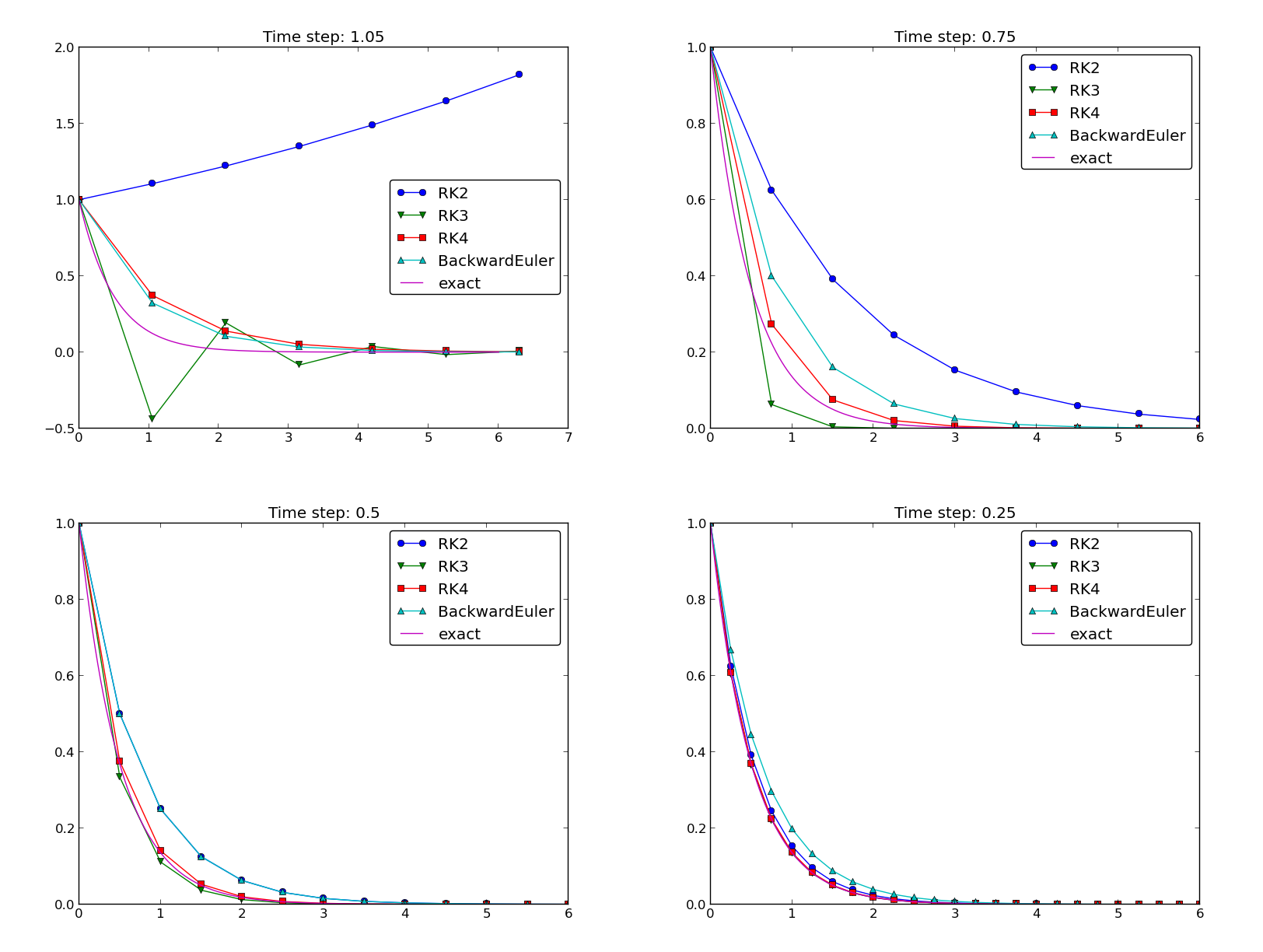
Behavior of different schemes for the decay equation
The runs in Figure Behavior of different schemes for the decay equation
and other experiments reveal that the 2nd-order Runge-Kutta
method (RK2) is unstable for \(\Delta t>1\) and decays slower than the
Backward Euler scheme for large and moderate \(\Delta t\) (see Exercise 3.5: Analyze explicit 2nd-order methods for an analysis). However, for
fine \(\Delta t = 0.25\) the 2nd-order Runge-Kutta method approaches
the exact solution faster than the Backward Euler scheme. That is,
the latter scheme does a better job for larger \(\Delta t\), while the
higher order scheme is superior for smaller \(\Delta t\). This is a
typical trend also for most schemes for ordinary and partial
differential equations.
The 3rd-order Runge-Kutta method (RK3) also has artifacts in the form
of oscillatory behavior for the larger \(\Delta t\) values, much
like that of the Crank-Nicolson scheme. For finer \(\Delta t\),
the 3rd-order Runge-Kutta method converges quickly to the exact
solution.
The 4th-order Runge-Kutta method (RK4) is slightly inferior
to the Backward Euler scheme on the coarsest mesh, but is then
clearly superior to all the other schemes. It is definitely the
method of choice for all the tested schemes.
Remark about using the \(\theta\)-rule in Odespy
The Odespy package assumes that the ODE is written as \(u^{\prime}=f(u,t)\) with an \(f\) that is possibly nonlinear in \(u\). The \(\theta\)-rule for \(u^{\prime}=f(u,t)\) leads to
which is a nonlinear equation in \(u^{n+1}\). Odespy’s implementation
of the \(\theta\)-rule (ThetaRule) and the specialized Backward Euler
(BackwardEuler) and Crank-Nicolson (CrankNicolson) schemes
must invoke iterative methods for
solving the nonlinear equation in \(u^{n+1}\). This is done even when
\(f\) is linear in \(u\), as in the model problem \(u^{\prime}=-au\), where we can
easily solve for \(u^{n+1}\) by hand. Therefore, we need to specify
use of Newton’s method to solve the equations.
(Odespy allows other methods than Newton’s to be used, for instance
Picard iteration, but that method is not suitable. The reason is that it
applies the Forward Euler scheme to generate a start value for
the iterations. Forward Euler may give very wrong solutions
for large \(\Delta t\) values. Newton’s method, on the other hand,
is insensitive to the start value in linear problems.)
Example: Adaptive Runge-Kutta methods
Odespy also offers solution methods that can adapt the size of \(\Delta t\) with time to match a desired accuracy in the solution. Intuitively, small time steps will be chosen in areas where the solution is changing rapidly, while larger time steps can be used where the solution is slowly varying. Some kind of error estimator is used to adjust the next time step at each time level.
A very popular adaptive method for solving ODEs is the Dormand-Prince
Runge-Kutta method of order 4 and 5. The 5th-order method is used as a
reference solution and the difference between the 4th- and 5th-order
methods is used as an indicator of the error in the numerical
solution. The Dormand-Prince method is the default choice in MATLAB’s
widely used ode45 routine.
We can easily set up Odespy to use the Dormand-Prince method and see how it selects the optimal time steps. To this end, we request only one time step from \(t=0\) to \(t=T\) and ask the method to compute the necessary non-uniform time mesh to meet a certain error tolerance. The code goes like
import odespy
import numpy as np
import decay_mod
import sys
#import matplotlib.pyplot as plt
import scitools.std as plt

def f(u, t):
    return -a*u

def u_exact(t):
    return I*np.exp(-a*t)

I = 1; a = 2; T = 5
tol = float(sys.argv[1])
solver = odespy.DormandPrince(f, atol=tol, rtol=0.1*tol)

Nt = 1  # just one step - let the scheme find its intermediate points
t_mesh = np.linspace(0, T, Nt+1)
t_fine = np.linspace(0, T, 10001)

solver.set_initial_condition(I)
u, t = solver.solve(t_mesh)

# u and t will only consist of [I, u^Nt] and [0,T]
# solver.u_all and solver.t_all contains all computed points
plt.plot(solver.t_all, solver.u_all, 'ko')
plt.hold('on')
plt.plot(t_fine, u_exact(t_fine), 'b-')
plt.legend(['tol=%.0E' % tol, 'exact'])
plt.savefig('tmp_odespy_adaptive.png')
plt.show()
Running four cases with tolerances \(10^{-1}\), \(10^{-3}\), \(10^{-5}\), and \(10^{-7}\), gives the results in Figure Choice of adaptive time mesh by the Dormand-Prince method for different tolerances. Intuitively, one would expect denser points in the beginning of the decay and larger time steps when the solution flattens out.
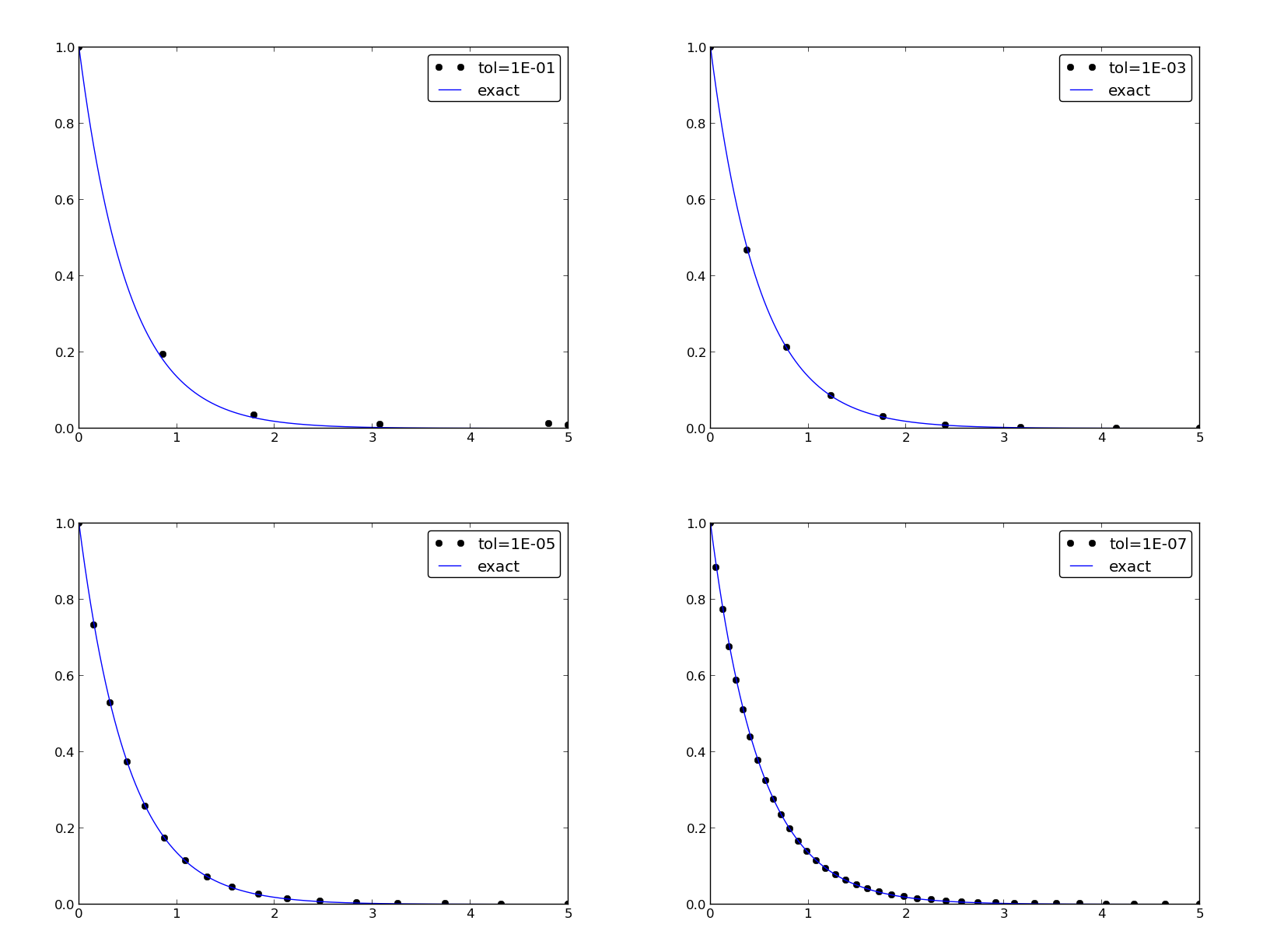
Choice of adaptive time mesh by the Dormand-Prince method for different tolerances
Exercises
Exercise 3.1: Experiment with precision in tests and the size of \(u\)
It is claimed in the section Verification via manufactured solutions that most numerical methods will
reproduce a linear exact solution to machine precision. Test this
assertion using the test function test_linear_solution in the
decay_vc.py program.
Vary the parameter c from very small, via c=1 to many larger values,
and print out the maximum difference between the numerical solution
and the exact solution. What is the relevant value of the tolerance
in the float comparison in each case?
Filename: test_precision.
Exercise 3.2: Implement the 2-step backward scheme
Implement the 2-step backward method (112) for the model \(u^{\prime}(t) = -a(t)u(t) + b(t)\), \(u(0)=I\). Allow the first step to be computed by either the Backward Euler scheme or the Crank-Nicolson scheme. Verify the implementation by choosing \(a(t)\) and \(b(t)\) such that the exact solution is linear in \(t\) (see the section Verification via manufactured solutions). Show mathematically that a linear solution is indeed a solution of the discrete equations.
Compute convergence rates (see the section Computing convergence rates) in
a test case using \(a=\hbox{const}\) and \(b=0\), where we easily have an exact
solution, and determine if the choice of a first-order scheme
(Backward Euler) for the first step has any impact on the overall
accuracy of this scheme. The expected error goes like \({\mathcal{O}(\Delta t^2)}\).
Filename: decay_backward2step.
Exercise 3.3: Implement the 2nd-order Adams-Bashforth scheme
Implement the 2nd-order Adams-Bashforth method (119)
for the decay problem \(u^{\prime}=-a(t)u + b(t)\), \(u(0)=I\), \(t\in (0, T]\).
Use the Forward Euler method for the first step such that the overall
scheme is explicit. Verify the implementation using an exact
solution that is linear in time.
Analyze the scheme by searching for solutions \(u^n=A^n\) when \(a=\hbox{const}\)
and \(b=0\). Compare this second-order scheme to the Crank-Nicolson scheme.
Filename: decay_AdamsBashforth2.
Exercise 3.4: Implement the 3rd-order Adams-Bashforth scheme
Implement the 3rd-order Adams-Bashforth method (120)
for the decay problem \(u^{\prime}=-a(t)u + b(t)\), \(u(0)=I\), \(t\in (0, T]\).
Since the scheme is explicit, allow it to be started by two steps with
the Forward Euler method. Investigate experimentally the case where
\(b=0\) and \(a\) is a constant: Can we have oscillatory solutions for
large \(\Delta t\)?
Filename: decay_AdamsBashforth3.
Exercise 3.5: Analyze explicit 2nd-order methods
Show that the schemes (117) and
(118) are identical in the case \(f(u,t)=-a\), where
\(a>0\) is a constant. Assume that the numerical solution reads
\(u^n=A^n\) for some unknown amplification factor \(A\) to be determined.
Find \(A\) and derive stability criteria. Can the scheme produce
oscillatory solutions of \(u^{\prime}=-au\)? Plot the numerical and exact
amplification factor.
Filename: decay_RK2_Taylor2.
Project 3.6: Implement and investigate the Leapfrog scheme
A Leapfrog scheme for the ODE \(u^{\prime}(t) = -a(t)u(t) + b(t)\) is defined by
A separate method is needed to compute \(u^1\). The Forward Euler scheme is a possible candidate.
a) Implement the Leapfrog scheme for the model equation. Plot the solution in the case \(a=1\), \(b=0\), \(I=1\), \(\Delta t = 0.01\), \(t\in [0,4]\). Compare with the exact solution \({u_{\small\mbox{e}}}(t)=e^{-t}\).
b) Show mathematically that a linear solution in \(t\) fulfills the Forward Euler scheme for the first step and the Leapfrog scheme for the subsequent steps. Use this linear solution to verify the implementation, and automate the verification through a test function.
Hint.
It can be wise to automate the calculations such that it is easy to
redo the calculations for other types of solutions. Here is
a possible sympy function that takes a symbolic expression u
(implemented as a Python function of t), fits the b term, and
checks if u fulfills the discrete equations:
import sympy as sym

def analyze(u):
    t, dt, a = sym.symbols('t dt a')

    print 'Analyzing u_e(t)=%s' % u(t)
    print 'u(0)=%s' % u(t).subs(t, 0)

    # Fit source term to the given u(t)
    b = sym.diff(u(t), t) + a*u(t)
    b = sym.simplify(b)
    print 'Source term b:', b

    # Residual in discrete equations; Forward Euler step
    R_step1 = (u(t+dt) - u(t))/dt + a*u(t) - b
    R_step1 = sym.simplify(R_step1)
    print 'Residual Forward Euler step:', R_step1

    # Residual in discrete equations; Leapfrog steps
    R = (u(t+dt) - u(t-dt))/(2*dt) + a*u(t) - b
    R = sym.simplify(R)
    print 'Residual Leapfrog steps:', R

def u_e(t):
    return c*t + I

analyze(u_e)
# or short form: analyze(lambda t: c*t + I)
c) Show that a second-order polynomial in \(t\) cannot be a solution of the discrete equations. However, if a Crank-Nicolson scheme is used for the first step, a second-order polynomial solves the equations exactly.
d) Create a manufactured solution \(u(t)=\sin(t)\) for the ODE \(u^{\prime}=-au+b\). Compute the convergence rate of the Leapfrog scheme using this manufactured solution. The expected convergence rate of the Leapfrog scheme is \({\mathcal{O}(\Delta t^2)}\). Does the use of a 1st-order method for the first step impact the convergence rate?
e) Set up a set of experiments to demonstrate that the Leapfrog scheme (125) is associated with numerical artifacts (instabilities). Document the main results from this investigation.
f) Analyze and explain the instabilities of the Leapfrog scheme (125):
- Choose \(a=\mbox{const}\) and \(b=0\). Assume that an exact solution of the discrete equations has the form \(u^n=A^n\), where \(A\) is an amplification factor to be determined. Derive an equation for \(A\) by inserting \(u^n=A^n\) in the Leapfrog scheme.
- Compute \(A\) either by hand and/or with the aid of
sympy. The polynomial for \(A\) has two roots, \(A_1\) and \(A_2\). Let \(u^n\) be a linear combination \(u^n=C_1A_1^n + C_2A_2^n\). - Show that one of the roots is the reason for instability.
- Compare \(A\) with the exact expression, using a Taylor series approximation.
- How can \(C_1\) and \(C_2\) be determined?
g) Since the original Leapfrog scheme is unconditionally unstable as time grows, it demands some stabilization. This can be done by filtering, where we first find \(u^{n+1}\) from the original Leapfrog scheme and then replace \(u^{n}\) by \(u^n + \gamma (u^{n-1} - 2u^n + u^{n+1})\), where \(\gamma\) can be taken as 0.6. Implement the filtered Leapfrog scheme and check that it can handle tests where the original Leapfrog scheme is unstable.
Filename: decay_leapfrog.
Problem 3.7: Make a unified implementation of many schemes
Consider the linear ODE problem \(u^{\prime}(t)=-a(t)u(t) + b(t)\), \(u(0)=I\). Explicit schemes for this problem can be written in the general form
for some choice of \(c_0,\ldots,c_m\). Find expressions for the \(c_j\) coefficients in case of the \(\theta\)-rule, the three-level backward scheme, the Leapfrog scheme, the 2nd-order Runge-Kutta method, and the 3rd-order Adams-Bashforth scheme.
Make a class ExpDecay that implements the
general updating formula (126).
The formula cannot be applied for \(n < m\), and for those \(n\) values, other
schemes must be used. Assume for simplicity that we just
repeat Crank-Nicolson steps until (126) can be used.
Use a subclass
to specify the list \(c_0,\ldots,c_m\) for a particular method, and
implement subclasses for all the mentioned schemes.
Verify the implementation by testing with a linear solution, which should
be exactly reproduced by all methods.
Filename: decay_schemes_unified.
