Analysis
We address the ODE for exponential decay,
where \(a\) and \(I\) are given constants. This problem is solved by the \(\theta\)-rule finite difference scheme, resulting in the recursive equations
for the numerical solution \(u^{n+1}\), which approximates the exact solution \({u_{\small\mbox{e}}}\) at time point \(t_{n+1}\). For constant mesh spacing, which we assume here, \(t_{n+1}=(n+1)\Delta t\).
The example programs associated with this chapter are found in the directory src/analysis.
Experimental investigations
We first perform a series of numerical explorations to see how the methods behave as we change the parameters \(I\), \(a\), and \(\Delta t\) in the problem.
Discouraging numerical solutions
Choosing \(I=1\), \(a=2\), and running experiments with \(\theta =1,0.5, 0\) for \(\Delta t=1.25, 0.75, 0.5, 0.1\), gives the results in Figures Backward Euler, Crank-Nicolson, and Forward Euler.
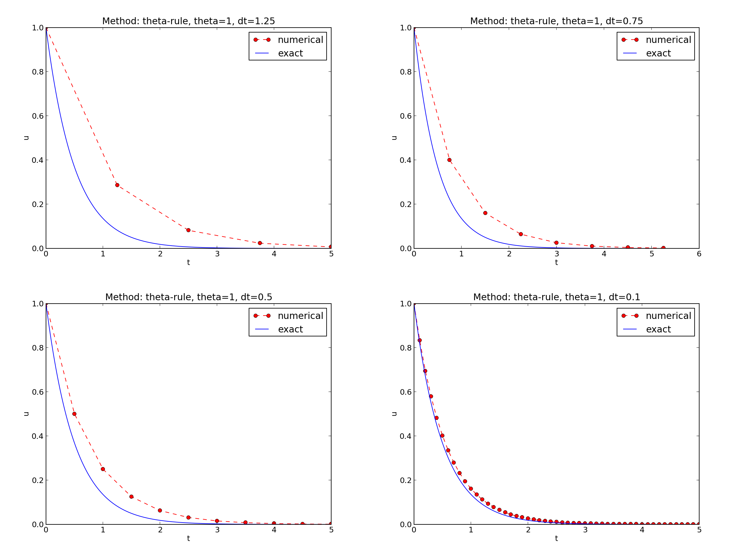
Backward Euler
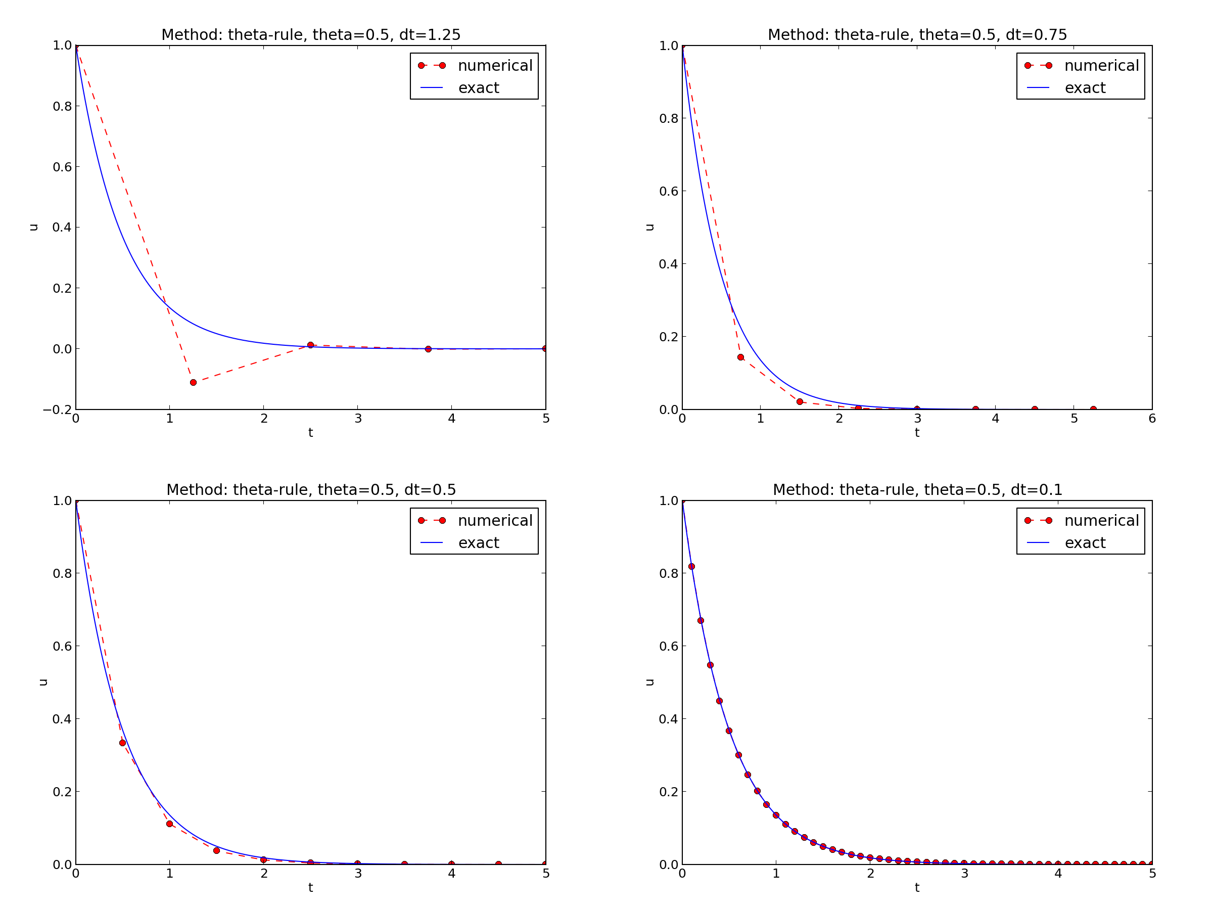
Crank-Nicolson
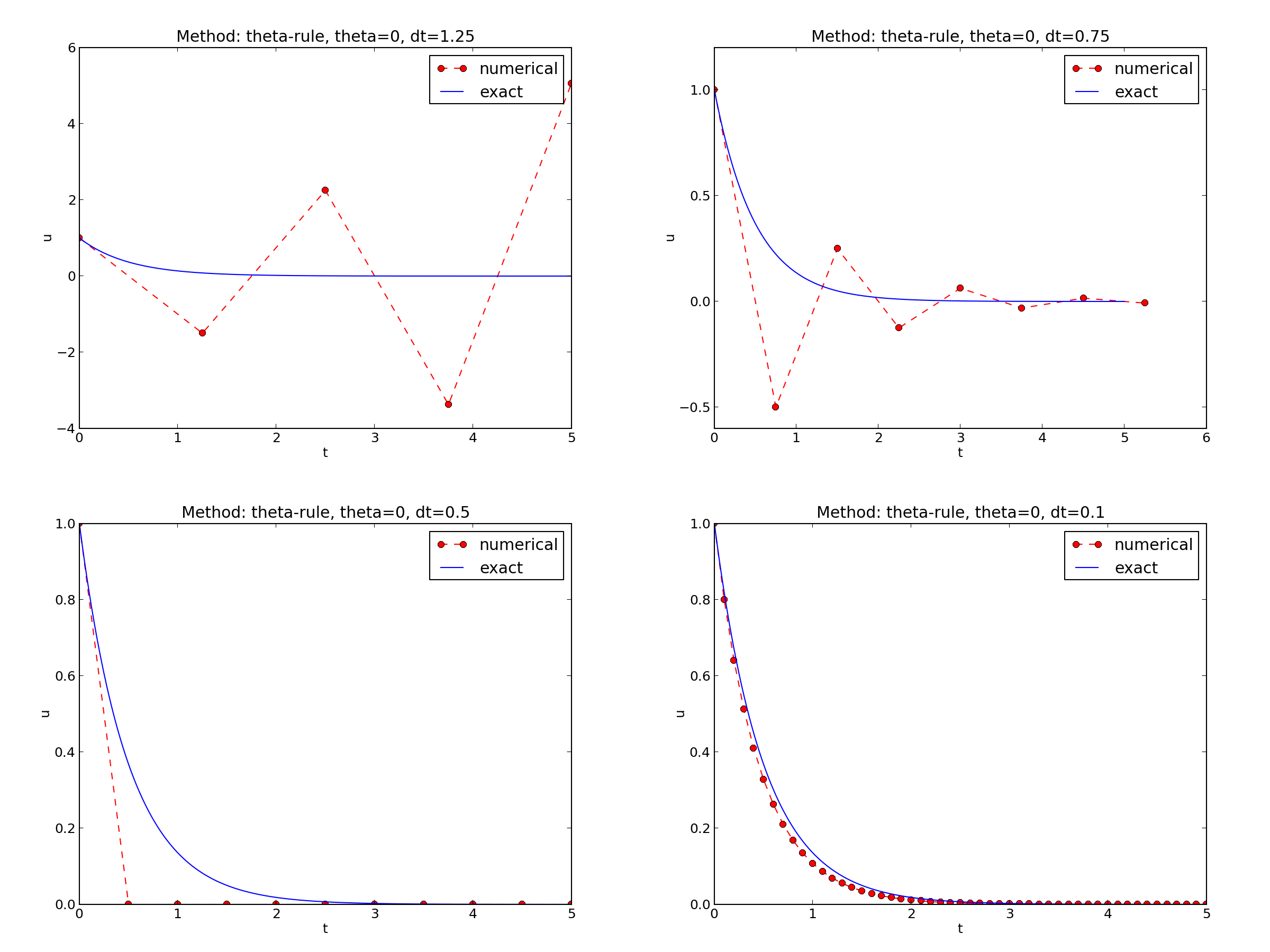
Forward Euler
The characteristics of the displayed curves can be summarized as follows:
- The Backward Euler scheme gives a monotone solution in all cases, lying above the exact curve.
- The Crank-Nicolson scheme gives the most accurate results, but for \(\Delta t=1.25\) the solution oscillates.
- The Forward Euler scheme gives a growing, oscillating solution for \(\Delta t=1.25\); a decaying, oscillating solution for \(\Delta t=0.75\); a strange solution \(u^n=0\) for \(n\geq 1\) when \(\Delta t=0.5\); and a solution seemingly as accurate as the one by the Backward Euler scheme for \(\Delta t = 0.1\), but the curve lies below the exact solution.
Since the exact solution of our model problem is a monotone function, \(u(t)=Ie^{-at}\), some of these qualitatively wrong results indeed seem alarming!
Key questions
- Under what circumstances, i.e., values of the input data \(I\), \(a\), and \(\Delta t\) will the Forward Euler and Crank-Nicolson schemes result in undesired oscillatory solutions?
- How does \(\Delta t\) impact the error in the numerical solution?
The first question will be investigated both by numerical experiments and by precise mathematical theory. The theory will help establish general criteria on \(\Delta t\) for avoiding non-physical oscillatory or growing solutions.
For our simple model problem we can answer the second question very precisely, but we will also look at simplified formulas for small \(\Delta t\) and touch upon important concepts such as convergence rate and the order of a scheme. Other fundamental concepts mentioned are stability, consistency, and convergence.
Detailed experiments
To address the first question above, we may set up an experiment where we loop over values of \(I\), \(a\), and \(\Delta t\) in our chosen model problem. For each experiment, we flag the solution as oscillatory if
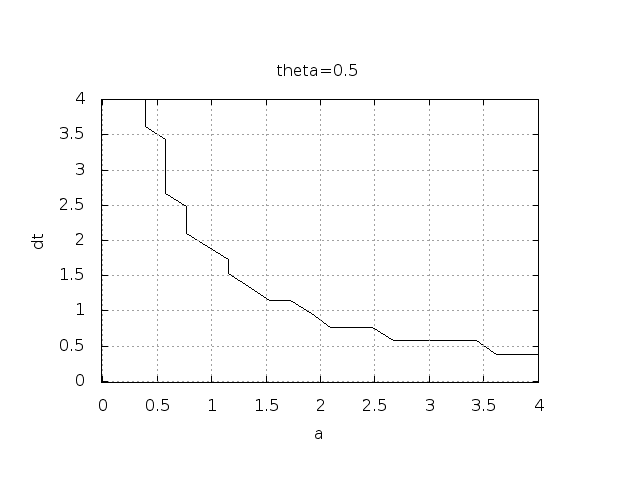
for some value of \(n\). This seems like a reasonable choice, since we expect \(u^n\) to decay with \(n\), but oscillations will make \(u\) increase over a time step. Doing some initial experimentation with varying \(I\), \(a\), and \(\Delta t\), quickly reveals that oscillations are independent of \(I\), but they do depend on \(a\) and \(\Delta t\). We can therefore limit the investigation to vary \(a\) and \(\Delta t\). Based on this observation, we introduce a two-dimensional function \(B(a,\Delta t)\) which is 1 if oscillations occur and 0 otherwise. We can visualize \(B\) as a contour plot (lines for which \(B=\hbox{const}\)). The contour \(B=0.5\) corresponds to the borderline between oscillatory regions with \(B=1\) and monotone regions with \(B=0\) in the \(a,\Delta t\) plane.
The \(B\) function is defined at discrete \(a\) and \(\Delta t\) values.
Say we have given \(P\) values for \(a\), \(a_0,\ldots,a_{P-1}\), and
\(Q\) values for \(\Delta t\), \(\Delta t_0,\ldots,\Delta t_{Q-1}\).
These \(a_i\) and \(\Delta t_j\) values, \(i=0,\ldots,P-1\),
\(j=0,\ldots,Q-1\), form a rectangular mesh of \(P\times Q\) points
in the plane spanned by \(a\) and \(\Delta t\).
At each point \((a_i, \Delta t_j)\), we associate
the corresponding value \(B(a_i,\Delta t_j)\), denoted \(B_{ij}\).
The \(B_{ij}\) values are naturally stored in a two-dimensional
array. We can thereafter create a plot of the
contour line \(B_{ij}=0.5\) dividing the oscillatory and monotone
regions. The file decay_osc_regions.py given below (osc_regions stands for “oscillatory regions”) contains all nuts and
bolts to produce the \(B=0.5\) line in Figures Forward Euler scheme: oscillatory solutions occur for points above the curve
and Crank-Nicolson scheme: oscillatory solutions occur for points above the curve. The oscillatory region is above this line.
from decay_mod import solver
import numpy as np
import scitools.std as st

def non_physical_behavior(I, a, T, dt, theta):
    """
    Given lists/arrays a and dt, and numbers I, dt, and theta,
    make a two-dimensional contour line B=0.5, where B=1>0.5
    means oscillatory (unstable) solution, and B=0<0.5 means
    monotone solution of u'=-au.
    """
    a = np.asarray(a); dt = np.asarray(dt)  # must be arrays
    B = np.zeros((len(a), len(dt)))         # results
    for i in range(len(a)):
        for j in range(len(dt)):
            u, t = solver(I, a[i], T, dt[j], theta)
            # Does u have the right monotone decay properties?
            correct_qualitative_behavior = True
            for n in range(1, len(u)):
                if u[n] > u[n-1]:  # Not decaying?
                    correct_qualitative_behavior = False
                    break  # Jump out of loop
            B[i,j] = float(correct_qualitative_behavior)
    a_, dt_ = st.ndgrid(a, dt)  # make mesh of a and dt values
    st.contour(a_, dt_, B, 1)
    st.grid('on')
    st.title('theta=%g' % theta)
    st.xlabel('a'); st.ylabel('dt')
    st.savefig('osc_region_theta_%s.png' % theta)
    st.savefig('osc_region_theta_%s.pdf' % theta)

non_physical_behavior(
    I=1,
    a=np.linspace(0.01, 4, 22),
    dt=np.linspace(0.01, 4, 22),
    T=6,
    theta=0.5)
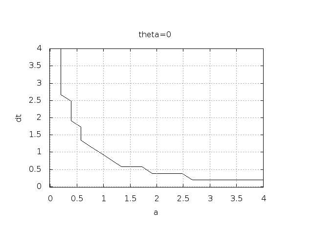
Forward Euler scheme: oscillatory solutions occur for points above the curve
Crank-Nicolson scheme: oscillatory solutions occur for points above the curve
By looking at the curves in the figures one may guess that \(a\Delta t\) must be less than a critical limit to avoid the undesired oscillations. This limit seems to be about 2 for Crank-Nicolson and 1 for Forward Euler. We shall now establish a precise mathematical analysis of the discrete model that can explain the observations in our numerical experiments.
Stability
The goal now is to understand the results in the previous section. To this end, we shall investigate the properties of the mathematical formula for the solution of the equations arising from the finite difference methods.
Exact numerical solution
Starting with \(u^0=I\), the simple recursion (60) can be applied repeatedly \(n\) times, with the result that
Solving difference equations
Difference equations where all terms are linear in \(u^{n+1}\), \(u^n\), and maybe \(u^{n-1}\), \(u^{n-2}\), etc., are called homogeneous, linear difference equations, and their solutions are generally of the form \(u^n=A^n\), where \(A\) is a constant to be determined. Inserting this expression in the difference equation and dividing by \(A^{n+1}\) gives a polynomial equation in \(A\). In the present case we get
This is a solution technique of wider applicability than repeated use of the recursion (60).
Regardless of the solution approach, we have obtained a formula for \(u^n\). This formula can explain everything we see in the figures above, but it also gives us a more general insight into accuracy and stability properties of the three schemes.
Since \(u^n\) is a factor \(A\) raised to an integer power \(n\), we realize that \(A < 0\) will imply \(u^n < 0\) for odd \(n\) and \(u^n > 0\) for even \(n\). That is, the solution oscillates between the mesh points. We have oscillations due to \(A < 0\) when
Since \(A>0\) is a requirement for having a numerical solution with the same basic property (monotonicity) as the exact solution, we may say that \(A>0\) is a stability criterion. Expressed in terms of \(\Delta t\) the stability criterion reads
The Backward Euler scheme is always stable since \(A < 0\) is impossible for \(\theta=1\), while non-oscillating solutions for Forward Euler and Crank-Nicolson demand \(\Delta t\leq 1/a\) and \(\Delta t\leq 2/a\), respectively. The relation between \(\Delta t\) and \(a\) look reasonable: a larger \(a\) means faster decay and hence a need for smaller time steps.
Looking at the upper left plot in Figure Forward Euler, we see that \(\Delta t=1.25\), and remembering that \(a=2\) in these experiments, \(A\) can be calculated to be \(-1.5\), so the Forward Euler solution becomes \(u^n=(-1.5)^n\) (\(I=1\)). This solution oscillates and grows. The upper right plot has \(a\Delta t = 2\cdot 0.75=1.5\), so \(A=-0.5\), and \(u^n=(-0.5)^n\) decays but oscillates. The lower left plot is a peculiar case where the Forward Euler scheme produces a solution that is stuck on the \(t\) axis. Now we can understand why this is so, because \(a\Delta t= 2\cdot 0.5=1\), which gives \(A=0\), and therefore \(u^n=0\) for \(n\geq 1\). The decaying oscillations in the Crank-Nicolson scheme in the upper left plot in Figure Crank-Nicolson for \(\Delta t=1.25\) are easily explained by the fact that \(A\approx -0.11 < 0\).
Stability properties derived from the amplification factor
The factor \(A\) is called the amplification factor since the solution at a new time level is the solution at the previous time level amplified by a factor \(A\). For a decay process, we must obviously have \(|A|\leq 1\), which is fulfilled for all \(\Delta t\) if \(\theta \geq 1/2\). Arbitrarily large values of \(u\) can be generated when \(|A|>1\) and \(n\) is large enough. The numerical solution is in such cases totally irrelevant to an ODE modeling decay processes! To avoid this situation, we must demand \(|A|\leq 1\) also for \(\theta < 1/2\), which implies
For example, \(\Delta t\) must not exceed \(2/a\) when computing with the Forward Euler scheme.
Stability properties
We may summarize the stability investigations as follows:
- The Forward Euler method is a conditionally stable scheme because it requires \(\Delta t < 2/a\) for avoiding growing solutions and \(\Delta t < 1/a\) for avoiding oscillatory solutions.
- The Crank-Nicolson is unconditionally stable with respect to growing solutions, while it is conditionally stable with the criterion \(\Delta t < 2/a\) for avoiding oscillatory solutions.
- The Backward Euler method is unconditionally stable with respect to growing and oscillatory solutions - any \(\Delta t\) will work.
Much literature on ODEs speaks about L-stable and A-stable methods. In our case A-stable methods ensures non-growing solutions, while L-stable methods also avoids oscillatory solutions.
Accuracy
While stability concerns the qualitative properties of the numerical solution, it remains to investigate the quantitative properties to see exactly how large the numerical errors are.
Visual comparison of amplification factors
After establishing how \(A\) impacts the qualitative features of the solution, we shall now look more into how well the numerical amplification factor approximates the exact one. The exact solution reads \(u(t)=Ie^{-at}\), which can be rewritten as
From this formula we see that the exact amplification factor is
We see from all of our analysis that the exact and numerical amplification factors depend on \(a\) and \(\Delta t\) through the dimensionless product \(a\Delta t\): whenever there is a \(\Delta t\) in the analysis, there is always an associated \(a\) parameter. Therefore, it is convenient to introduce a symbol for this product, \(p=a\Delta t\), and view \(A\) and \({A_{\small\mbox{e}}}\) as functions of \(p\). Figure Comparison of amplification factors shows these functions. The two amplification factors are clearly closest for the Crank-Nicolson method, but that method has the unfortunate oscillatory behavior when \(p>2\).
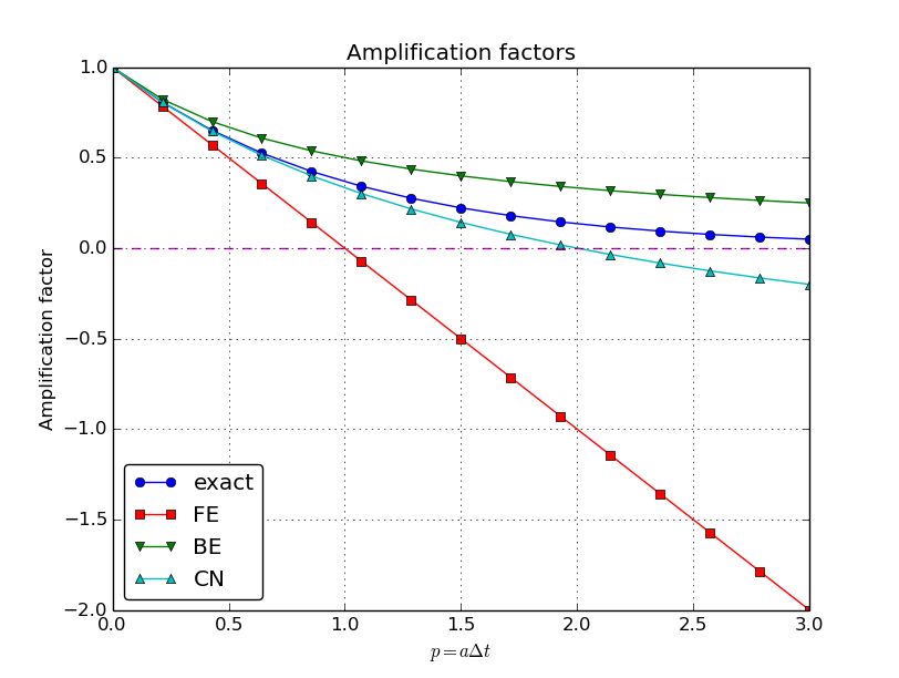
Comparison of amplification factors
Significance of the \(p=a\Delta t\) parameter
The key parameter for numerical performance of a scheme is in this model problem \(p=a\Delta t\). This is a dimensionless number (\(a\) has dimension 1/s and \(\Delta t\) has dimension s) reflecting how the discretization parameter plays together with a physical parameter in the problem.
One can bring the present model problem on dimensionless form through a process called scaling. The scaled modeled has a modified time \(\bar t = at\) and modified response \(\bar u =u/I\) such that the model reads \(d\bar u/d\bar t = -\bar u\), \(\bar u(0)=1\). Analyzing this model, where there are no physical parameters, we find that \(\Delta \bar t\) is the key parameter for numerical performance. In the unscaled model, this corresponds to \(\Delta \bar t = a\Delta t\).
It is common that the numerical performance of methods for solving ordinary and partial differential equations is governed by dimensionless parameters that combine mesh sizes with physical parameters.
Series expansion of amplification factors
As an alternative to the visual understanding inherent in Figure Comparison of amplification factors, there is a strong tradition in numerical analysis to establish formulas for approximation errors when the discretization parameter, here \(\Delta t\), becomes small. In the present case, we let \(p\) be our small discretization parameter, and it makes sense to simplify the expressions for \(A\) and \({A_{\small\mbox{e}}}\) by using Taylor polynomials around \(p=0\). The Taylor polynomials are accurate for small \(p\) and greatly simplify the comparison of the analytical expressions since we then can compare polynomials, term by term.
Calculating the Taylor series for \({A_{\small\mbox{e}}}\) is easily done by hand, but
the three versions of \(A\) for \(\theta=0,1,{\frac{1}{2}}\) lead to more
cumbersome calculations.
Nowadays, analytical computations can benefit greatly by
symbolic computer algebra software. The Python package sympy
represents a powerful computer algebra system, not yet as sophisticated as
the famous Maple and Mathematica systems, but it is free and
very easy to integrate with our numerical computations in Python.
When using sympy, it is convenient to enter an interactive Python
shell where the results of expressions and statements can be shown
immediately.
Here is a simple example. We strongly recommend to use
isympy (or ipython) for such interactive sessions.
Let us illustrate sympy with a standard Python shell syntax
(>>> prompt) to compute a Taylor polynomial approximation to \(e^{-p}\):
>>> from sympy import *
>>> # Create p as a mathematical symbol with name 'p'
>>> p = Symbols('p')
>>> # Create a mathematical expression with p
>>> A_e = exp(-p)
>>>
>>> # Find the first 6 terms of the Taylor series of A_e
>>> A_e.series(p, 0, 6)
1 + (1/2)*p**2 - p - 1/6*p**3 - 1/120*p**5 + (1/24)*p**4 + O(p**6)
Lines with >>> represent input lines, whereas without
this prompt represent the result of the previous command (note that
isympy and ipython apply other prompts, but in this text
we always apply >>> for interactive Python computing).
Apart from the order of the powers, the computed formula is easily
recognized as the beginning of the Taylor series for \(e^{-p}\).
Let us define the numerical amplification factor where \(p\) and \(\theta\) enter the formula as symbols:
>>> theta = Symbol('theta')
>>> A = (1-(1-theta)*p)/(1+theta*p)
To work with the factor for the Backward Euler scheme we
can substitute the value 1 for theta:
>>> A.subs(theta, 1)
1/(1 + p)
Similarly, we can substitute theta by 1/2 for Crank-Nicolson,
preferably using an exact rational representation of 1/2 in sympy:
>>> half = Rational(1,2)
>>> A.subs(theta, half)
1/(1 + (1/2)*p)*(1 - 1/2*p)
The Taylor series of the amplification factor for the Crank-Nicolson scheme can be computed as
>>> A.subs(theta, half).series(p, 0, 4)
1 + (1/2)*p**2 - p - 1/4*p**3 + O(p**4)
We are now in a position to compare Taylor series:
>>> FE = A_e.series(p, 0, 4) - A.subs(theta, 0).series(p, 0, 4)
>>> BE = A_e.series(p, 0, 4) - A.subs(theta, 1).series(p, 0, 4)
>>> CN = A_e.series(p, 0, 4) - A.subs(theta, half).series(p, 0, 4 )
>>> FE
(1/2)*p**2 - 1/6*p**3 + O(p**4)
>>> BE
-1/2*p**2 + (5/6)*p**3 + O(p**4)
>>> CN
(1/12)*p**3 + O(p**4)
From these expressions we see that the error \(A-{A_{\small\mbox{e}}}\sim {\mathcal{O}(p^2)}\) for the Forward and Backward Euler schemes, while \(A-{A_{\small\mbox{e}}}\sim {\mathcal{O}(p^3)}\) for the Crank-Nicolson scheme. The notation \({\mathcal{O}(p^m)}\) here means a polynomial in \(p\) where \(p^m\) is the term of lowest-degree, and consequently the term that dominates the expression for \(p < 0\). We call this the leading order term. As \(p\rightarrow 0\), the leading order term clearly dominates over the higher-order terms (think of \(p=0.01\): \(p\) is a hundred times larger than \(p^2\)).
Now, \(a\) is a given parameter in the problem, while \(\Delta t\) is what we can vary. Not surprisingly, the error expressions are usually written in terms \(\Delta t\). We then have
We say that the Crank-Nicolson scheme has an error in the amplification factor of order \(\Delta t^3\), while the two other schemes are of order \(\Delta t^2\) in the same quantity.
What is the significance of the order expression? If we halve \(\Delta t\), the error in amplification factor at a time level will be reduced by a factor of 4 in the Forward and Backward Euler schemes, and by a factor of 8 in the Crank-Nicolson scheme. That is, as we reduce \(\Delta t\) to obtain more accurate results, the Crank-Nicolson scheme reduces the error more efficiently than the other schemes.
The ratio of numerical and exact amplification factors
An alternative comparison of the schemes is provided by looking at the ratio \(A/{A_{\small\mbox{e}}}\), or the error \(1-A/{A_{\small\mbox{e}}}\) in this ratio:
>>> FE = 1 - (A.subs(theta, 0)/A_e).series(p, 0, 4)
>>> BE = 1 - (A.subs(theta, 1)/A_e).series(p, 0, 4)
>>> CN = 1 - (A.subs(theta, half)/A_e).series(p, 0, 4)
>>> FE
(1/2)*p**2 + (1/3)*p**3 + O(p**4)
>>> BE
-1/2*p**2 + (1/3)*p**3 + O(p**4)
>>> CN
(1/12)*p**3 + O(p**4)
The leading-order terms have the same powers as in the analysis of \(A-{A_{\small\mbox{e}}}\).
The global error at a point
The error in the amplification factor reflects the error when
progressing from time level \(t_n\) to \(t_{n-1}\) only. That is,
we disregard the error already present in the solution at \(t_{n-1}\).
The real error at a point, however, depends on the error development
over all previous time steps. This error,
\(e^n = u^n-{u_{\small\mbox{e}}}(t_n)\), is known as the global error. We
may look at \(u^n\) for some \(n\) and Taylor expand the
mathematical expressions as functions of \(p=a\Delta t\) to get a simple
expression for the global error (for small \(p\)). Continuing the
sympy expression from previous section, we can write
>>> n = Symbol('n')
>>> u_e = exp(-p*n)
>>> u_n = A**n
>>> FE = u_e.series(p, 0, 4) - u_n.subs(theta, 0).series(p, 0, 4)
>>> BE = u_e.series(p, 0, 4) - u_n.subs(theta, 1).series(p, 0, 4)
>>> CN = u_e.series(p, 0, 4) - u_n.subs(theta, half).series(p, 0, 4)
>>> FE
(1/2)*n*p**2 - 1/2*n**2*p**3 + (1/3)*n*p**3 + O(p**4)
>>> BE
(1/2)*n**2*p**3 - 1/2*n*p**2 + (1/3)*n*p**3 + O(p**4)
>>> CN
(1/12)*n*p**3 + O(p**4)
Note that sympy does not sort the polynomial terms in the output,
so \(p^3\) appears before \(p^2\) in the output of BE.
For a fixed time \(t\), the parameter \(n\) in these expressions increases as \(p\rightarrow 0\) since \(t=n\Delta t =\mbox{const}\) and hence \(n\) must increase like \(\Delta t^{-1}\). With \(n\) substituted by \(t/\Delta t\) in the leading-order error terms, these become
The global error is therefore of second order (in \(\Delta t\)) for the Crank-Nicolson scheme and of first order for the other two schemes.
Convergence
When the global error \(e^n\rightarrow 0\) as \(\Delta t\rightarrow 0\), we say that the scheme is convergent. It means that the numerical solution approaches the exact solution as the mesh is refined, and this is a much desired property of a numerical method.
Integrated error
It is common to study the norm of the numerical error, as
explained in detail in the section Computing the norm of the error mesh function.
The \(L^2\) norm of the error can be computed by treating \(e^n\) as a function
of \(t\) in sympy and performing symbolic integration.
From now on we shall do import sympy as sym and prefix all functions
in sympy by sym to explicitly notify ourselves that the functions
are from sympy. This is particularly advantageous when we use
mathematical functions like sin: sym.sin is for symbolic expressions,
while sin from numpy or math is for numerical computation.
For the Forward Euler scheme we have
import sympy as sym
p, n, a, dt, t, T, theta = sym.symbols('p n a dt t T theta')
A = (1-(1-theta)*p)/(1+theta*p)
u_e = sym.exp(-p*n)
u_n = A**n
error = u_e.series(p, 0, 4) - u_n.subs(theta, 0).series(p, 0, 4)
# Introduce t and dt instead of n and p
error = error.subs('n', 't/dt').subs(p, 'a*dt')
error = error.as_leading_term(dt) # study only the first term
print error
error_L2 = sym.sqrt(sym.integrate(error**2, (t, 0, T)))
print 'L2 error:', sym.simplify(error_error_L2)
The output reads
sqrt(30)*sqrt(T**3*a**4*dt**2*(6*T**2*a**2 - 15*T*a + 10))/60
which means that the \(L^2\) error behaves like \(a^2\Delta t\).
Strictly speaking, the numerical error is only defined at the mesh points so it makes most sense to compute the \(\ell^2\) error
We have obtained an exact analytical expression for the error at \(t=t_n\), but here we use the leading-order error term only since we are mostly interested in how the error behaves as a polynomial in \(\Delta t\) or \(p\), and then the leading order term will dominate. For the Forward Euler scheme, \({u_{\small\mbox{e}}}(t_n) - u^n \approx {\frac{1}{2}}np^2\), and we have
Now, \(\sum_{n=0}^{N_t} n^2\approx \frac{1}{3}N_t^3\). Using this approximation, setting \(N_t =T/\Delta t\), and taking the square root gives the expression
Calculations for the Backward Euler scheme are very similar and provide the same result, while the Crank-Nicolson scheme leads to
Truncation error
The truncation error is a very frequently used error measure for finite difference methods. It is defined as the error in the difference equation that arises when inserting the exact solution. Contrary to many other error measures, e.g., the true error \(e^n={u_{\small\mbox{e}}}(t_n)-u^n\), the truncation error is a quantity that is easily computable.
Before reading on, it is wise to review the section Mathematical derivation of finite difference formulas on how Taylor polynomials were used to derive finite differences and quantify the error in the formulas. Very similar reasoning, and almost identical mathematical details, will be carried out below, but in a slightly different context. Now, the focus is on the error when solving a differential equation, while in the section Mathematical derivation of finite difference formulas we derived errors for a finite difference formula. These errors are tightly connected in the present model problem.
Let us illustrate the calculation of the truncation error for the Forward Euler scheme. We start with the difference equation on operator form,
which is the short form for
The idea is to see how well the exact solution \({u_{\small\mbox{e}}}(t)\) fulfills this equation. Since \({u_{\small\mbox{e}}}(t)\) in general will not obey the discrete equation, we get an error in the discrete equation. This error is called a residual, denoted here by \(R^n\):
The residual is defined at each mesh point and is therefore a mesh function with a superscript \(n\).
The interesting feature of \(R^n\) is to see how it depends on the discretization parameter \(\Delta t\). The tool for reaching this goal is to Taylor expand \({u_{\small\mbox{e}}}\) around the point where the difference equation is supposed to hold, here \(t=t_n\). We have that
which may be used to reformulate the fraction in (73) so that
Now, \({u_{\small\mbox{e}}}\) fulfills the ODE \({u_{\small\mbox{e}}}'=-a{u_{\small\mbox{e}}}\), which means that the first and last term cancel and we have
This \(R^n\) is the truncation error, which for the Forward Euler is seen to be of first order in \(\Delta t\) as \(\Delta \rightarrow 0\).
The above procedure can be repeated for the Backward Euler and the Crank-Nicolson schemes. We start with the scheme in operator notation, write it out in detail, Taylor expand \({u_{\small\mbox{e}}}\) around the point \(\tilde t\) at which the difference equation is defined, collect terms that correspond to the ODE (here \({u_{\small\mbox{e}}}' + a{u_{\small\mbox{e}}}\)), and identify the remaining terms as the residual \(R\), which is the truncation error. The Backward Euler scheme leads to
while the Crank-Nicolson scheme gives
when \(\Delta t\rightarrow 0\).
The order \(r\) of a finite difference scheme is often defined through the leading term \(\Delta t^r\) in the truncation error. The above expressions point out that the Forward and Backward Euler schemes are of first order, while Crank-Nicolson is of second order. We have looked at other error measures in other sections, like the error in amplification factor and the error \(e^n={u_{\small\mbox{e}}}(t_n)-u^n\), and expressed these error measures in terms of \(\Delta t\) to see the order of the method. Normally, calculating the truncation error is more straightforward than deriving the expressions for other error measures and therefore the easiest way to establish the order of a scheme.
Consistency, stability, and convergence
Three fundamental concepts when solving differential equations by numerical methods are consistency, stability, and convergence. We shall briefly touch upon these concepts below in the context of the present model problem.
Consistency means that the error in the difference equation, measured through the truncation error, goes to zero as \(\Delta t\rightarrow 0\). Since the truncation error tells how well the exact solution fulfills the difference equation, and the exact solution fulfills the differential equation, consistency ensures that the difference equation approaches the differential equation in the limit. The expressions for the truncation errors in the previous section are all proportional to \(\Delta t\) or \(\Delta t^2\), hence they vanish as \(\Delta t\rightarrow 0\), and all the schemes are consistent. Lack of consistency implies that we actually solve some other differential equation in the limit \(\Delta t\rightarrow 0\) than we aim at.
Stability means that the numerical solution exhibits the same qualitative properties as the exact solution. This is obviously a feature we want the numerical solution to have. In the present exponential decay model, the exact solution is monotone and decaying. An increasing numerical solution is not in accordance with the decaying nature of the exact solution and hence unstable. We can also say that an oscillating numerical solution lacks the property of monotonicity of the exact solution and is also unstable. We have seen that the Backward Euler scheme always leads to monotone and decaying solutions, regardless of \(\Delta t\), and is hence stable. The Forward Euler scheme can lead to increasing solutions and oscillating solutions if \(\Delta t\) is too large and is therefore unstable unless \(\Delta t\) is sufficiently small. The Crank-Nicolson can never lead to increasing solutions and has no problem to fulfill that stability property, but it can produce oscillating solutions and is unstable in that sense, unless \(\Delta t\) is sufficiently small.
Convergence implies that the global (true) error mesh function \(e^n = {u_{\small\mbox{e}}}(t_n)-u^n\rightarrow 0\) as \(\Delta t\rightarrow 0\). This is really what we want: the numerical solution gets as close to the exact solution as we request by having a sufficiently fine mesh.
Convergence is hard to establish theoretically, except in quite simple problems like the present one. Stability and consistency are much easier to calculate. A major breakthrough in the understanding of numerical methods for differential equations came in 1956 when Lax and Richtmeyer established equivalence between convergence on one hand and consistency and stability on the other (the Lax equivalence theorem). In practice it meant that one can first establish that a method is stable and consistent, and then it is automatically convergent (which is much harder to establish). The result holds for linear problems only, and in the world of nonlinear differential equations the relations between consistency, stability, and convergence are much more complicated.
We have seen in the previous analysis that the Forward Euler, Backward Euler, and Crank-Nicolson schemes are convergent (\(e^n\rightarrow 0\)), that they are consistent (\(R^n\rightarrow 0\)), and that they are stable under certain conditions on the size of \(\Delta t\). We have also derived explicit mathematical expressions for \(e^n\), the truncation error, and the stability criteria.
Various types of errors in a differential equation model
So far we have been concerned with one type of error, namely the discretization error committed by replacing the differential equation problem by a recursive set of difference equations. There are, however, other types of errors that must be considered too. We can classify errors into four groups:
- model errors: how wrong is the ODE model?
- data errors: how wrong are the input parameters?
- discretization errors: how wrong is the numerical method?
- rounding errors: how wrong is the computer arithmetics?
Below, we shall briefly describe and illustrate these four types of errors. Each of the errors deserve its own chapter, at least, so the treatment here is superficial to give some indication about the nature of size of the errors in a specific case. Some of the required computer codes quickly become more advanced than in the rest of the book, but we include to code to document all the details that lie behind the investigations of the errors.
Model errors
Any mathematical model like \(u^{\prime}=-au\), \(u(0)=I\), is just an approximate description of a real-world phenomenon. How good this approximation is can be determined by comparing physical experiments with what the model predicts. This is the topic of validation and is obviously an essential part of mathematical model. One difficulty with validation is that we need to estimate the parameters in the model, and this brings in data errors. Quantifying data errors is challenging, and a frequently used method is to tune the parameters in the model to make model predictions as close as possible to the experiments. That is, we do not attempt to measure or estimate all input parameters, but instead find values that “make the model good”. Another difficulty is that the response in experiments also contains errors due to measurement techniques.
Let us try to quantify model errors in a very simple example involving \(u^{\prime}=-au\), \(u(0)=I\), with constant \(a\). Suppose a more accurate model has \(a\) as a function of time rather than a constant. Here we take \(a(t)\) as a simple linear function: \(a + pt\). Obviously, \(u\) with \(p>0\) will go faster to zero with time than a constant \(a\).
The solution of
can be shown (see below) to be
Let a Python function true_model(t, I, a, p) implement the
above \(u(t)\) and let
the solution of our primary ODE \(u^{\prime}=-au\) be available as
the function model(t, I, a).
We can now make some plots of the two models and the error for some values
of \(p\). Figure Comparison of two models for three values of displays
model versus true_model for \(p=0.01, 0.1, 1\), while Figure
Discrepancy of Comparison of two models for three values of shows the difference
between the two models as a function of \(t\) for the same \(p\) values.
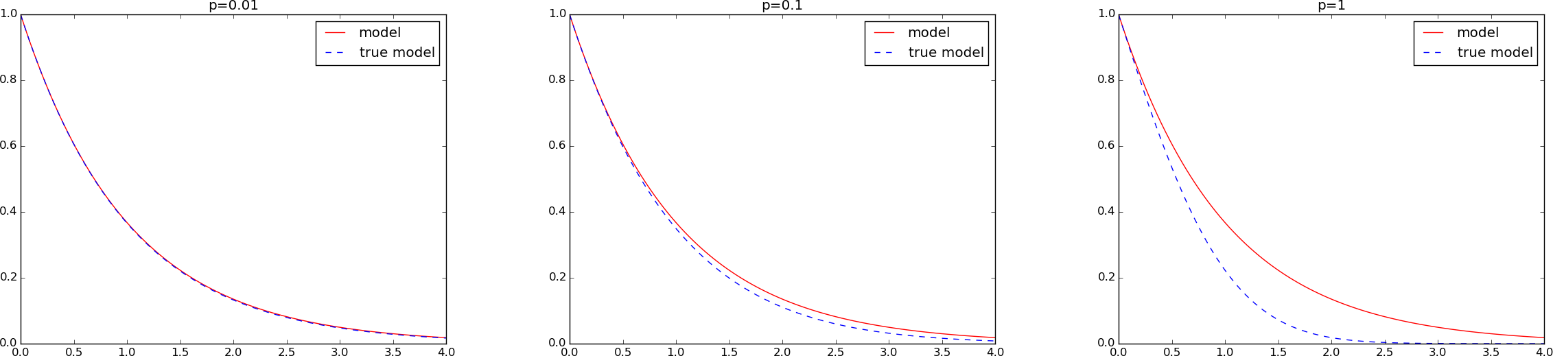
Comparison of two models for three values of \(p\)
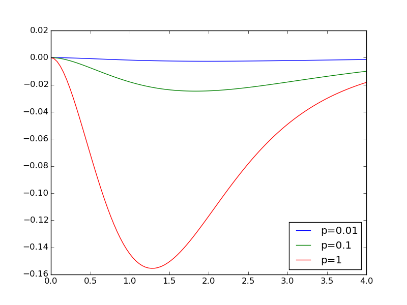
Discrepancy of Comparison of two models for three values of \(p\)
The code that was used to produce the plots looks like
from numpy import linspace, exp
from matplotlib.pyplot import \
     plot, show, xlabel, ylabel, legend, savefig, figure, title

def model_errors():
    p_values = [0.01, 0.1, 1]
    a = 1
    I = 1
    t = linspace(0, 4, 101)
    legends = []
    # Work with figure(1) for the discrepancy and figure(2+i)
    # for plotting the model and the true model for p value no i
    for i, p in enumerate(p_values):
        u = model(t, I, a)
        u_true = true_model(t, I, a, p)
        discrepancy = u_true - u
        figure(1)
        plot(t, discrepancy)
        figure(2+i)
        plot(t, u, 'r-', t, u_true, 'b--')
        legends.append('p=%g' % p)
    figure(1)
    legend(legends, loc='lower right')
    savefig('tmp1.png'); savefig('tmp1.pdf')
    for i, p in enumerate(p_values):
        figure(2+i)
        legend(['model', 'true model'])
        title('p=%g' % p)
        savefig('tmp%d.png' % (2+i)); savefig('tmp%d.pdf' % (2+i))
To derive the analytical solution of the model \(u^{\prime}=-(a+pt)u\), \(u(0)=I\), we can use SymPy and the code below. This is somewhat advanced SymPy use for a newbie, but serves to illustrate the possibilities to solve differential equations by symbolic software.
def derive_true_solution():
    import sympy as sym
    u = sym.symbols('u', cls=sym.Function)  # function u(t)
    t, a, p, I = sym.symbols('t a p I', real=True)

    def ode(u, t, a, p):
        """Define ODE: u' = (a + p*t)*u. Return residual."""
        return sym.diff(u, t) + (a + p*t)*u

    eq = ode(u(t), t, a, p)
    s = sym.dsolve(eq)
    # s is sym.Eq object u(t) == expression, we want u = expression,
    # so grab the right-hand side of the equality (Eq obj.)
    u = s.rhs
    print u
    # u contains C1, replace it with a symbol we can fit to
    # the initial condition
    C1 = sym.symbols('C1', real=True)
    u = u.subs('C1', C1)
    print u
    # Initial condition equation
    eq = u.subs(t, 0) - I
    s = sym.solve(eq, C1)  # solve eq wrt C1
    print s
    # s is a list s[0] = ...
    # Replace C1 in u by the solution
    u = u.subs(C1, s[0])
    print 'u:', u
    print sym.latex(u)  # latex formula for reports

    # Consistency check: u must fulfill ODE and initial condition
    print 'ODE is fulfilled:', sym.simplify(ode(u, t, a, p))
    print 'u(0)-I:', sym.simplify(u.subs(t, 0) - I)

    # Convert u expression to Python numerical function
    # (modules='numpy' allows numpy arrays as arguments,
    # we want this for t)
    u_func = sym.lambdify([t, I, a, p], u, modules='numpy')
    return u_func

true_model = derive_true_solution()
Data errors
By “data” we mean all the input parameters to a model, in our case \(I\) and \(a\). The values of these may contain errors, or at least uncertainty. Suppose \(I\) and \(a\) are measured from some physical experiments. Ideally, we have many samples of \(I\) and \(a\) and from these we can fit probability distributions. Assume that \(I\) turns out to be normally distributed with mean 1 and standard deviation 0.2, while \(a\) is uniformly distributed in the interval \([0.5, 1.5]\).
How will the uncertainty in \(I\) and \(a\) propagate through the model \(u=Ie^{-at}\)? That is, what is the uncertainty in \(u\) at a particular time \(t\)? This answer can easily be answered using Monte Carlo simulation. It means that we draw a lot of samples from the distributions for \(I\) and \(a\). For each combination of \(I\) and \(a\) sample we compute the corresponding \(u\) value for selected values of \(t\). Afterwards, we can for each selected \(t\) values make a histogram of all the computed \(u\) values to see what the distribution of \(u\) values look like. Figure Histogram of solution uncertainty at three time points, due to data errors shows the histograms corresponding to \(t=0,1,3\). We see that the distribution of \(u\) values is much like a symmetric normal distribution at \(t=0\), centered around \(u=1\). At later times, the distribution gets more asymmetric and narrower. It means that the uncertainty decreases with time.
From the computed \(u\) values we can easily calculate the mean and standard deviation. The table below shows the mean and standard deviation values along with the value if we just use the formula \(u=Ie^{-at}\) with the mean values of \(I\) and \(a\): \(I=1\) and \(a=1\). As we see, there is some discrepancy between this latter (naive) computation and the mean value produced by Monte Carlo simulation.
| time | mean | st.dev. | \(u(t;I=a=1)\) |
|---|---|---|---|
| 0 | 1.00 | 0.200 | 1.00 |
| 1 | 0.38 | 0.135 | 0.37 |
| 3 | 0.07 | 0.060 | 0.14 |
Actually, \(u(t;I,a)\) becomes a stochastic variable for each \(t\) when \(I\) and \(a\) are stochastic variables, as they are in the above Monte Carlo simulation. The mean of the stochastic \(u(t;I,a)\) is not equal to \(u\) with mean values of the input data, \(u(t;I=a=1)\), unless \(u\) is linear in \(I\) and \(a\) (here \(u\) is nonlinear in \(a\)).
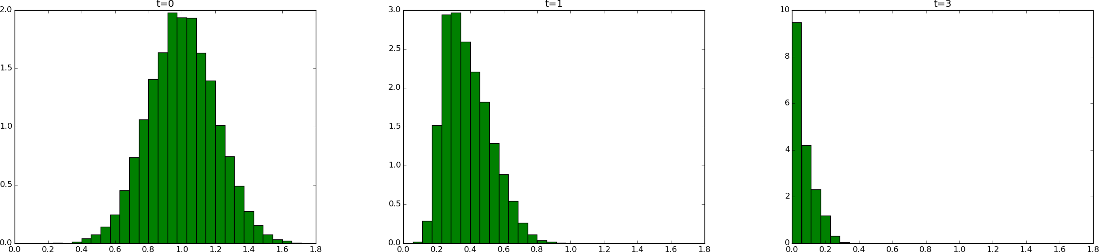
Histogram of solution uncertainty at three time points, due to data errors
Estimating statistical uncertainty in input data and investigating how this uncertainty propagates to uncertainty in the response of a differential equation model (or other models) are key topics in the scientific field called uncertainty quantification, simply known as UQ. Estimation of the statistical properties of input data can either be done directly from physical experiments, or one can find the parameter values that provide a “best fit” of model predictions with experiments. Monte Carlo simulation is a general and widely used tool to solve the associated statistical problems. The accuracy of the Monte Carlo results increases with increasing number of samples \(N\), typically the error behaves like \(N^{-1/2}\).
The computer code required to do the Monte Carlo simulation and produce the plots in Figure Histogram of solution uncertainty at three time points, due to data errors is shown below.
def data_errors():
    from numpy import random, mean, std
    from matplotlib.pyplot import hist
    N = 10000
    # Draw random numbers for I and a
    I_values = random.normal(1, 0.2, N)
    a_values = random.uniform(0.5, 1.5, N)
    # Compute corresponding u values for some t values
    t = [0, 1, 3]
    u_values = {}  # samples for various t values
    u_mean = {}
    u_std = {}
    for t_ in t:
        # Compute u samples corresponding to I and a samples
        u_values[t_] = [model(t_, I, a)
                        for I, a in zip(I_values, a_values)]
        u_mean[t_] = mean(u_values[t_])
        u_std[t_] = std(u_values[t_])

        figure()
        dummy1, bins, dummy2 = hist(
            u_values[t_], bins=30, range=(0, I_values.max()),
            normed=True, facecolor='green')
        #plot(bins)
        title('t=%g' % t_)
        savefig('tmp_%g.png' % t_); savefig('tmp_%g.pdf' % t_)
    # Table of mean and standard deviation values
    print 'time   mean   st.dev.'
    for t_ in t:
        print '%3g    %.2f    %.3f' % (t_, u_mean[t_], u_std[t_])
Discretization errors
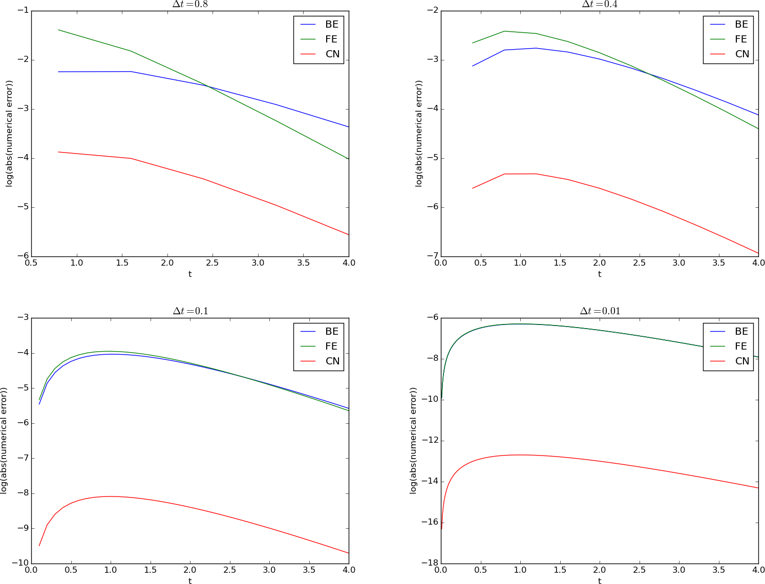
The errors implied by solving the differential equation problem by the \(\theta\)-rule has been thoroughly analyzed in the previous sections. Below are some plots of the error versus time for the Forward Euler (FE), Backward Euler (BN), and Crank-Nicolson (CN) schemes for decreasing values of \(\Delta t\). Since the difference in magnitude between the errors in the CN scheme versus the FE and BN schemes grows significantly as \(\Delta t\) is reduced (the error goes like \(\Delta t^2\) for CN versus \(\Delta t\) for FE/BE), we have plotted the logarithm of the absolute value of the numerical error as a mesh function.
Discretization errors in various schemes for four time step values
The table below presents exact figures of the discretization error for various choices of \(\Delta t\) and schemes.
| \(\Delta t\) | FE | BE | CN |
|---|---|---|---|
| 0.4 | \(9\cdot 10^{-2}\) | \(6\cdot 10^{-2}\) | $ 5cdot 10^{-3}$ |
| 0.1 | \(2\cdot 10^{-2}\) | \(2\cdot 10^{-2}\) | $ 3cdot 10^{-4}$ |
| 0.01 | \(2\cdot 10^{-3}\) | \(2\cdot 10^{-3}\) | $ 3cdot 10^{-6}$ |
The computer code used to generate the plots appear next. It makes use
of a solver function
as shown in the section Integer division.
def discretization_errors():
    from numpy import log, abs
    I = 1
    a = 1
    T = 4
    t = linspace(0, T, 101)
    schemes = {'FE': 0, 'BE': 1, 'CN': 0.5}  # theta to scheme name
    dt_values = [0.8, 0.4, 0.1, 0.01]
    for dt in dt_values:
        figure()
        legends = []
        for scheme in schemes:
            theta = schemes[scheme]
            u, t = solver(I, a, T, dt, theta)
            u_e = model(t, I, a)
            error = u_e - u
            print '%s: dt=%.2f, %d steps, max error: %.2E' % \
                  (scheme, dt, len(u)-1, abs(error).max())
            # Plot log(error), but exclude error[0] since it is 0
            plot(t[1:], log(abs(error[1:])))
            legends.append(scheme)
        xlabel('t');  ylabel('log(abs(numerical error))')
        legend(legends, loc='upper right')
        title(r'$\Delta t=%g$' % dt)
        savefig('tmp_dt%g.png' % dt); savefig('tmp_dt%g.pdf' % dt)
Rounding errors
Real numbers on a computer are represented by floating-point numbers, which means that just a finite number of digits are stored and used. Therefore, the floating-point number is an approximation to the underlying real number. When doing arithmetics with floating-point numbers, there will be small approximation errors, called round-off errors or rounding errors, that may or may not accumulate in comprehensive computations.
The cause and analysis of rounding errors are described in most books on numerical analysis, see for instance Chapter 2 in Gander et al. [Ref05]. For very simple algorithms it is possible to theoretically establish bounds for the rounding errors, but for most algorithms one cannot know to what extent rounding errors accumulate and potentially destroy the final answer. Problem 2.3: Explore rounding errors in numerical calculus demonstrates the impact of rounding errors on numerical differentiation and integration.
Here is a simplest possible example of the effect of rounding errors:
>>> 1.0/51*51
1.0
>>> 1.0/49*49
0.9999999999999999
We see that the latter result is not exact, but features an error of
\(10^{-16}\). This is the typical level of a rounding error from an
arithmetic operation with the widely used 64 bit floating-point number
(float object in Python, often called double or double precision
in other languages). One cannot expect more accuracy than \(10^{-16}\).
The big question is if errors at this level accumulate in a given
numerical algorithm.
What is the effect of using float objects and not exact arithmetics
when solving differential equations? We can investigate this question
through computer experiments if we have the ability to represent real
numbers to a desired accuracy. Fortunately, Python has a Decimal
object in the decimal module that allows us
to use as many digits in floating-point numbers as we like. We take
1000 digits as the true answer where rounding errors are negligible,
and then we run our numerical algorithm (the Crank-Nicolson scheme to
be precise) with Decimal objects for all real numbers and compute
the maximum error arising from using 4, 16, 64, and 128 digits.
When computing with numbers around unity in size and doing \(N_t=40\) time steps, we typically get a rounding error of \(10^{-d}\), where \(d\) is the number of digits used. The effect of rounding errors may accumulate if we perform more operations, so increasing the number of time steps to 4000 gives a rounding error of the order \(10^{-d+2}\). Also, if we compute with numbers that are much larger than unity, we lose accuracy due to rounding errors. For example, for the \(u\) values implied by \(I=1000\) and \(a=100\) (\(u\sim 10^3\)), the rounding errors increase to about \(10^{-d+3}\). Below is a table summarizing a set of experiments. A rough model for the size of rounding errors is \(10^{-d+q+r}\), where \(d\) is the number of digits, the number of time steps is of the order \(10^q\) time steps, and the size of the numbers in the arithmetic expressions are of order \(10^r\).
| digits | \(u\sim 1\), \(N_t=40\) | \(u\sim 1\), \(N_t=4000\) | \(u\sim 10^3\), \(N_t=40\) | \(u\sim 10^3\), \(N_t=4000\) |
|---|---|---|---|---|
| 4 | \(3.05\cdot 10^{-4}\) | \(2.51\cdot 10^{-1}\) | \(3.05\cdot 10^{-1}\) | \(9.82\cdot 10^{2}\) |
| 16 | \(1.71\cdot 10^{-16}\) | \(1.42\cdot 10^{-14}\) | \(1.58\cdot 10^{-13}\) | \(4.84\cdot 10^{-11}\) |
| 64 | \(2.99\cdot 10^{-64}\) | \(1.80\cdot 10^{-62}\) | \(2.06\cdot 10^{-61}\) | \(1.04\cdot 10^{-57}\) |
| 128 | \(1.60\cdot 10^{-128}\) | \(1.56\cdot 10^{-126}\) | \(2.41\cdot 10^{-125}\) | \(1.07\cdot 10^{-122}\) |
We realize that rounding errors are at the lowest possible level if we scale the differential equation model, see the section Scaling, so the numbers entering the computations are of unity in size, and if we take a small number of steps (40 steps gives a discretization error of \(5\cdot 10^{-3}\) with the Crank-Nicolson scheme). In general, rounding errors are negligible in comparison with other errors in differential equation models.
The computer code for doing the reported experiments need a new version
of the solver function where we do arithmetics with Decimal
objects:
def solver_decimal(I, a, T, dt, theta):
    """Solve u'=-a*u, u(0)=I, for t in (0,T] with steps of dt."""
    from numpy import zeros, linspace
    from decimal import Decimal as D
    dt = D(dt)
    a = D(a)
    theta = D(theta)
    Nt = int(round(D(T)/dt))
    T = Nt*dt
    u = zeros(Nt+1, dtype=object)  # array of Decimal objects
    t = linspace(0, float(T), Nt+1)

    u[0] = D(I)               # assign initial condition
    for n in range(0, Nt):    # n=0,1,...,Nt-1
        u[n+1] = (1 - (1-theta)*a*dt)/(1 + theta*dt*a)*u[n]
    return u, t
The function below carries out the experiments. We can conveniently
set the number of digits as we want through the decimal.getcontext().prec
variable.
def rounding_errors(I=1, a=1, T=4, dt=0.1):
    import decimal
    from numpy import log, array, abs
    digits_values = [4, 16, 64, 128]
    # "Exact" arithmetics is taken as 1000 decimals here
    decimal.getcontext().prec = 1000
    u_e, t = solver_decimal(I=I, a=a, T=T, dt=dt, theta=0.5)
    for digits in digits_values:
        decimal.getcontext().prec = digits  # set no of digits
        u, t = solver_decimal(I=I, a=a, T=T, dt=dt, theta=0.5)
        error = u_e - u
        error = array(error[1:], dtype=float)
        print '%d digits, %d steps, max abs(error): %.2E' % \
              (digits, len(u)-1, abs(error).max())
Discussion of the size of various errors
The previous computational examples of model, data, discretization, and rounding errors are tied to one particular mathematical problem, so it is in principle dangerous to make general conclusions. However, the illustrations made point to some common trends that apply to differential equation models.
First, rounding errors have very little impact compared to the other types of errors. Second, numerical errors are in general smaller than model and data errors, but more importantly, numerical errors are often well understood and can be reduced by just increasing the computational work (in our example by taking more smaller time steps).
Third, data errors may be significant, and it also takes a significant amount of computational work to quantify them and their impact on the solution. Many types of input data are also difficult or impossible to measure, so finding suitable values requires tuning of the data and the model to a known (measured) response. Nevertheless, even if the predictive precision of a model is limited because of severe errors or uncertainty in input data, the model can still be of high value for investigating qualitative properties of the underlying phenomenon. Through computer experiments with synthetic input data one can understand a lot of the science or engineering that goes into the model.
Fourth, model errors are the most challenging type of error to deal with. Simplicity of model is in general preferred over complexity, but adding complexity is often the only way to improve the predictive capabilities of a model. More complexity usually also means a need for more input data and consequently the danger of increasing data errors.
Exercises
Problem 2.1: Visualize the accuracy of finite differences
The purpose of this exercise is to visualize the accuracy of finite difference approximations of the derivative of a given function. For any finite difference approximation, take the Forward Euler difference as an example, and any specific function, take \(u=e^{-at}\), we may introduce an error fraction
and view \(E\) as a function of \(\Delta t\). We expect that \(\lim_{\Delta t\rightarrow 0}E=1\), while \(E\) may deviate significantly from unity for large \(\Delta t\). How the error depends on \(\Delta t\) is best visualized in a graph where we use a logarithmic scale for \(\Delta t\), so we can cover many orders of magnitude of that quantity. Here is a code segment creating an array of 100 intervals, on the logarithmic scale, ranging from \(10^{-6}\) to \(10^{-0.5}\) and then plotting \(E\) versus \(p=a\Delta t\) with logarithmic scale on the \(p\) axis:
from numpy import logspace, exp
from matplotlib.pyplot import semilogx
p = logspace(-6, -0.5, 101)
y = (1-exp(-p))/p
semilogx(p, y)
Illustrate such errors for the finite difference operators \([D_t^+u]^n\) (forward), \([D_t^-u]^n\) (backward), and \([D_t u]^n\) (centered) in the same plot.
Perform a Taylor series expansions of the error fractions and find the leading order \(r\) in the expressions of type \(1 + Cp^r + {\mathcal{O}(p^{r+1)}}\), where \(C\) is some constant.
Hint.
To save manual calculations and learn more about symbolic computing,
make functions for the three difference operators and use sympy
to perform the symbolic differences, differentiation, and Taylor series
expansion. To plot a symbolic expression E against p, convert the
expression to a Python function first: E = sympy.lamdify([p], E).
Filename: decay_plot_fd_error.
Problem 2.2: Explore the \(\theta\)-rule for exponential growth
This exercise asks you to solve the ODE \(u'=-au\) with \(a < 0\) such that the ODE models exponential growth instead of exponential decay. A central theme is to investigate numerical artifacts and non-physical solution behavior.
a) Set \(a=-1\) and run experiments with \(\theta=0, 0.5, 1\) for various values of \(\Delta t\) to uncover numerical artifacts. Recall that the exact solution is a monotone, growing function when \(a < 0\). Oscillations or significantly wrong growth are signs of wrong qualitative behavior.
From the experiments, select four values of \(\Delta t\) that demonstrate the kind of numerical solutions that are characteristic for this model.
b) Write up the amplification factor and plot it for \(\theta=0,0.5,1\) together with the exact one for \(a\Delta t < 0\). Use the plot to explain the observations made in the experiments.
Hint.
Modify the decay_ampf_plot.py code
(in the src/analysis directory).
Filename: exponential_growth.
Problem 2.3: Explore rounding errors in numerical calculus
a) Compute the absolute values of the errors in the numerical derivative of \(e^{-t}\) at \(t=\frac{1}{2}\) for three types of finite difference approximations: a forward difference, a backward difference, and a centered difference, for \(\Delta t = 2^{-k}\), \(k=0,4, 8, 12, \ldots, 60\). When do rounding errors destroy the accuracy?
b) Compute the absolute values of the errors in the numerical approximation of \(\int_0^4 e^{-t}dt\) using the Trapezoidal and the Midpoint integration methods. Make a table of the errors for \(n=2^k\) intervals, \(k=1,3,5=ldots,21\). Is there any impact of rounding errors?
Hint. The Trapezoidal rule for \(\int_a^bf(x)dx\) reads
The Midpoint rule is
Filename: rounding.
