Demonstrations
Dirichlet and Neumann conditions: reflecting and mirroring boundaries
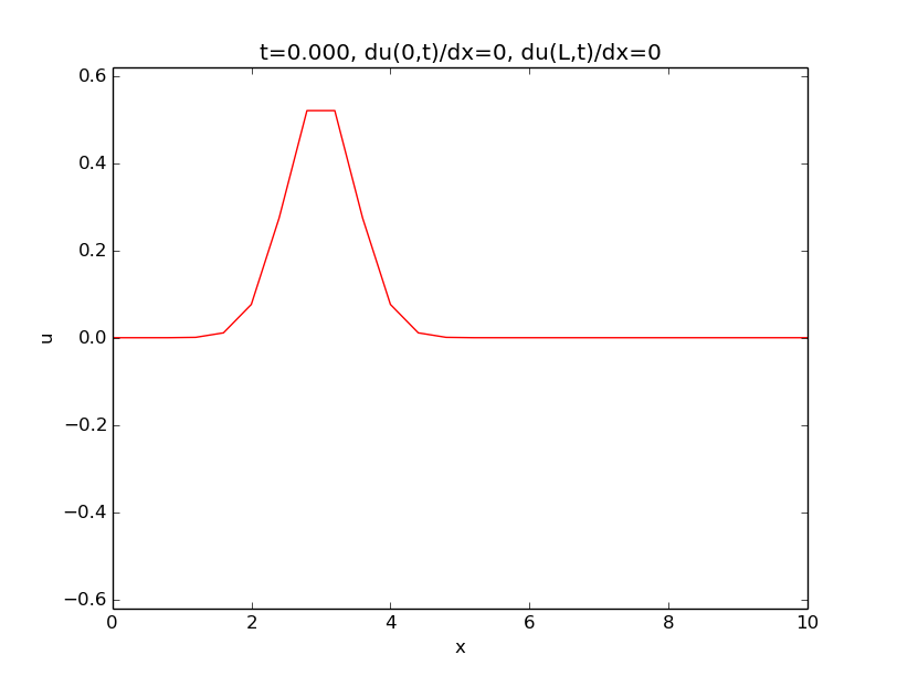
The first two animations demonstrates the differences between a Dirichlet condition \( u=0 \) at the boundary and a Neumann condition \( \partial u/\partial x=0 \).
Reflecting boundaries (\( u_x=0 \)) for a Gaussian wave.
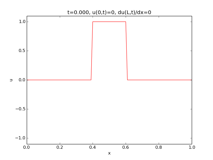
Mirroring boundaries (\( u=0 \)) for a Gaussian wave.
Instead of a Gaussian wave profile, we can test the geometrically simple plug profile.
Numerical noise
All of the above computations were run with unit Courant number, which means that the solutions are exact without any numerical errors. (This is a remarkable property of the numerical solution method.) For smaller Courant numbers, numerical noise may be visible, depending on the smoothness of the initial profile. Below is a smooth Gaussian profile and the almost discontinuous plug profile.
Reflecting boundaries (\( u_x=0 \)) for a Gaussian wave, computed with \( C=0.5 \), which implies numerical noise on a coarse grid.
A plug wave generates very significant numerical noise (\( C=0.5 \)).
Effect of impulsive start of waves
The previous demonstrations had an initial condition with a prescribed \( u=0 \) profile at rest (\( u_t=0 \)). Alternatively, one may start with a flat profile \( u=0 \) and use an initial condition \( u_t=V\neq 0 \) to impulsively start the wave motion. For example, if we think of \( u \) as the displacement of a string on a string instrument, this set of initial conditions corresponds to an undeformed string that is given an impulsive start from an impact.
Impulsive start of a wave motion: \( I=0 \), \( V\neq 0 \).
Feeding of waves from the boundary
We can also start with a flat profile, \( u=0 \), at rest, \( u_t=0 \), and create propagating signals by moving \( u \) at the boundary. That is, we have a time-varying Dirichlet condition \( u(0,t)=U_0(t) \) at the left boundary. The movements lead to signals that propagate to the right. In the movie, the movements are paused to make separate signals.
Feeding of waves from the boundary by a time-dependent Dirichlet condition \( U_0(t) \).
Open and periodic boundary conditions
Demonstrations of periodic boundary condition on the left combined with an open boundary condition on the right: waves passing out of the domain enter the left end again.
Demonstrations of periodic boundary condition on the left combined with an open boundary condition on the right: waves passing out of the domain enter the left end again.
Error in the open boundary condition
In 2D and 3D...
Periodic boundary condition combined with a slight wrong open boundary condition at the right end (20% wrong wave velocity leads to small reflections back into the domain).
| Condition | Formula | Effect |
| Dirichlet | \( u(0,t)=0 \) | mirror wave |
| Dirichlet | \( u(0,t)=U_0(t) \) | feed incoming wave |
| Neumann | \( u_x(0,t)=0 \) | reflect wave |
| Open | \( u_t \pm cu_x=0 \) | let wave out of the domain |
| Periodic | \( u(0,t)=u(L,t) \) | turn outgoing wave to incoming |
Science is a differential equation. Religion is a boundary condition. Alan Turing, computer scientist, 1912-1954.