Mathematical model and solution method

We solve a one-dimensional, linear, constant-coefficient wave equation by an explicit finite difference method.

The wave equation problem

The standard, linear wave equation in a homogeneous one-dimensional medium reads $$ \begin{equation} \frac{\partial^2 u}{\partial t^2} = c^2 \frac{\partial^2 u}{\partial x^2}, \quad x\in (0,L),\ t\in (0,T]\tp \tag{1} \end{equation} $$ The unknown function $ u $ depends on space $ x $ and time $ t $: $ u=u(x,t) $.

The need for boundary conditions in the wave equation. Four initial and boundary conditions must be specified to have a unique solution:

Initial condition for $ u(x,0) $
Initial condition for $ u_t(x,0) $
Boundary condition at $ x=0 $
Boundary condition at $ x=L $

Initial conditions

Most demonstrations will start with an initial profile of $ u $, $$ u(x,0) = I(x), $$ being at rest, i.e., $$ \frac{\partial}{\partial t}u(x,0) = 0\tp $$ Two initial profiles will be considered: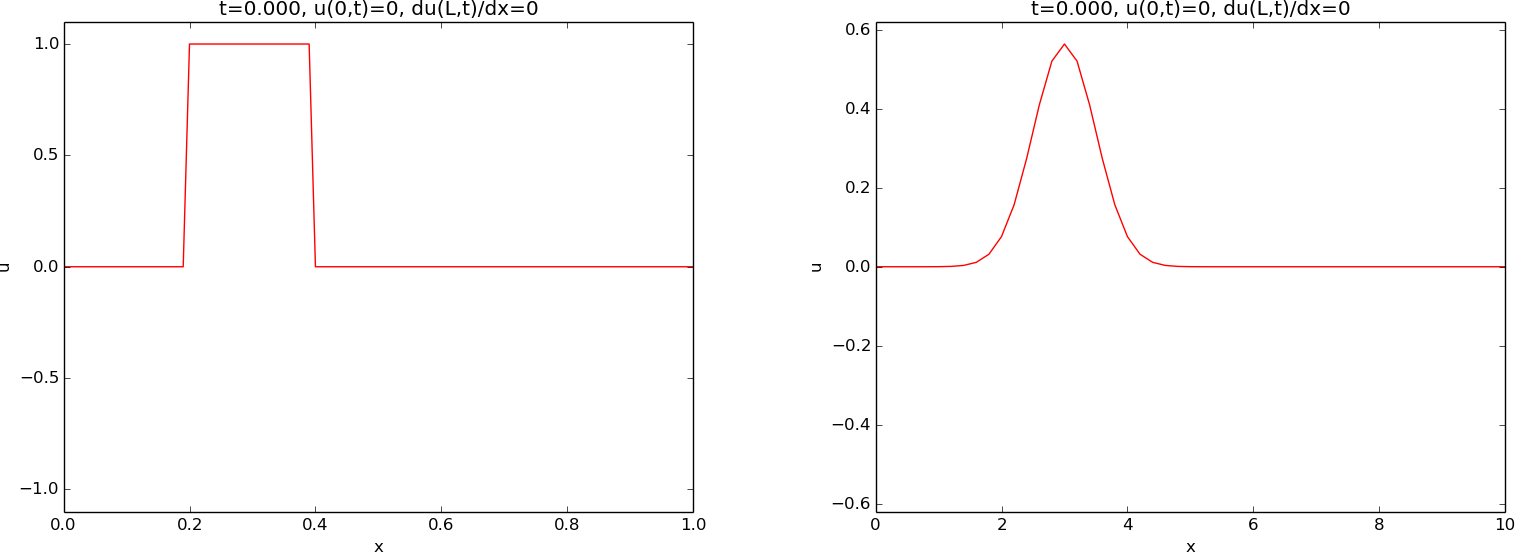

a plug as to left in Figure 1
a Gaussian peak as to the right in Figure 1

Figure 1: Examples on initial conditions.

Boundary conditions

Fixed $ u $

At $ x=0 $ we will sometimes use the condition $ u=0 $, often known as a homogeneous Dirichlet condition. This condition will mirror the wave.

Reflecting condition

At $ x=0 $ and/or $ x=L $ we will apply a reflecting or no-flux condition: $$ \begin{equation} \frac{\partial u}{\partial x}=0\tp \tag{2} \end{equation} $$ This condition reflects the wave into the domain again, as a surface wave hits a vertical wave, runs up to the double amplitude, and propagates back into the domain again. This type of boundary condition is also referred to as a Neumann condition.

Feeding a wave from the boundary

We shall demonstrate the effect of moving $ u $ at the boundary $ x=0 $ to feed the domain with an incoming wave. The boundary condition then reads $$ u(0,t) = U_0(t),$$ for some given function $ U_0(t) $. A particular choice in a later demonstration is a sine function that is active in three different time intervals: $$ U_0 (t) = \left\lbrace\begin{array}{ll} \frac{1}{4}\sin(6\pi t),& t\in T_1\hbox{ or } t\in T_2\hbox{ or } t\in T_3\\ 0,& \hbox{otherwise} \end{array}\right. $$ where $ T_1=[0, \frac{1}{6}] $, $ T_2=[\frac{3}{4}, \frac{5}{6}] $, and $ T_3=[\frac{3}{2},\frac{11}{6}] $. The movement of $ u $ at the boundary will produce a wave that is by the PDE transported to the right into the domain.

Open boundary condition

Very often one wants to let a wave travel through the boundary without being disturbed. Such a condition is called an open boundary condition, or a radiation condition, or an artificial boundary condition: $$ \begin{align} \frac{\partial u}{\partial t} - c\frac{\partial u}{\partial x} &= 0,\quad x=0, \tag{3}\\ \frac{\partial u}{\partial t} + c\frac{\partial u}{\partial x} &= 0,\quad x=L\tp \tag{4} \end{align} $$ These conditions work exactly in 1D, but are challenging to generalize and implement in 2D and 3D.

Periodic boundary condition

When following a wave motion over large distances, it is desireable to let a wave travel out of the right domain and at the same time feed the wave back into the domain from the left. This approach avoids a very large domain where nothing happens in the majority of the domain. A periodic boundary condition at $ x=0 $ can be used to feed the signal traveling out at $ x=L $ into the domain: $$ \begin{equation} u(0,t) = u(L,t)\tp \tag{5} \end{equation} $$ The condition at $ x=L $ is then an open boundary condition (4).

Numerical solution method

The wave equation is solved by an explicit finite difference method, which is of second-order in space and time. A uniform mesh with spacing $ \Delta x $ and $ \Delta t $ is used in space and time, respectively. The no-flux or Neumann boundary conditions are implemented by modifying the computational stencil at the boundary. The open boundary conditions are implemented by forward in time, upstream in space finite differences, which exactly let the wave out of the boundary. More details are found in Appendix: Numerical solution method. Parts of the computer code are explained in Appendix: Computer code.