Computing integrals

We now turn our attention to solving mathematical problems through computer programming. There are many reasons to choose integration as our first application. Integration is well known already from high school mathematics. Most integrals are not tractable by pen and paper, and a computerized solution approach is both very much simpler and much more powerful - you can essentially treat all integrals \(\int_a^bf(x)dx\) in 10 lines of computer code (!). Integration also demonstrates the difference between exact mathematics by pen and paper and numerical mathematics on a computer. The latter approaches the result of the former without any worries about rounding errors due to finite precision arithmetics in computers (in contrast to differentiation, where such errors prevent us from getting a result as accurate as we desire on the computer). Finally, integration is thought of as a somewhat difficult mathematical concept to grasp, and programming integration should greatly help with the understanding of what integration is and how it works. Not only shall we understand how to use the computer to integrate, but we shall also learn a series of good habits to ensure your computer work is of the highest scientific quality. In particular, we have a strong focus on how to write Python code that is free of programming mistakes.

Calculating an integral is traditionally done by

\[\tag{2} \int_a^b f(x)\,dx = F(b) - F(a),\]

where

\[f(x) = \frac{dF}{dx} \thinspace .\]

The major problem with this procedure is that we need to find the anti-derivative \(F(x)\) corresponding to a given \(f(x)\). For some relatively simple integrands \(f(x)\), finding \(F(x)\) is a doable task, but it can very quickly become challenging, even impossible!

The method (2) provides an exact or analytical value of the integral. If we relax the requirement of the integral being exact, and instead look for approximate values, produced by numerical methods, integration becomes a very straightforward task for any given \(f(x)\) (!).

The downside of a numerical method is that it can only find an approximate answer. Leaving the exact for the approximate is a mental barrier in the beginning, but remember that most real applications of integration will involve an \(f(x)\) function that contains physical parameters, which are measured with some error. That is, \(f(x)\) is very seldom exact, and then it does not make sense to compute the integral with a smaller error than the one already present in \(f(x)\).

Another advantage of numerical methods is that we can easily integrate a function \(f(x)\) that is only known as samples, i.e., discrete values at some \(x\) points, and not as a continuous function of \(x\) expressed through a formula. This is highly relevant when \(f\) is measured in a physical experiment.

Basic ideas of numerical integration

We consider the integral

\[\tag{3} \int_a^b f(x)dx\thinspace .\]

Most numerical methods for computing this integral split up the original integral into a sum of several integrals, each covering a smaller part of the original integration interval \([a,b]\). This re-writing of the integral is based on a selection of integration points \(x_i\), \(i = 0,1,\ldots,n\) that are distributed on the interval \([a,b]\). Integration points may, or may not, be evenly distributed. An even distribution simplifies expressions and is often sufficient, so we will mostly restrict ourselves to that choice. The integration points are then computed as

\[\tag{4} x_i = a + ih,\quad i = 0,1,\ldots,n,\]

where

\[\tag{5} h = \frac{b-a}{n}\thinspace .\]

Given the integration points, the original integral is re-written as a sum of integrals, each integral being computed over the sub-interval between two consecutive integration points. The integral in (3) is thus expressed as

\[\tag{6} \int_a^b f(x)dx = \int_{x_0}^{x_1} f(x)dx + \int_{x_1}^{x_2} f(x)dx + \ldots + \int_{x_{n-1}}^{x_n} f(x)dx\thinspace .\]

Note that \(x_0 = a\) and \(x_n = b\).

Proceeding from (6), the different integration methods will differ in the way they approximate each integral on the right hand side. The fundamental idea is that each term is an integral over a small interval \([x_i,x_{i+1}]\), and over this small interval, it makes sense to approximate \(f\) by a simple shape, say a constant, a straight line, or a parabola, which we can easily integrate by hand. The details will become clear in the coming examples.

Computational example

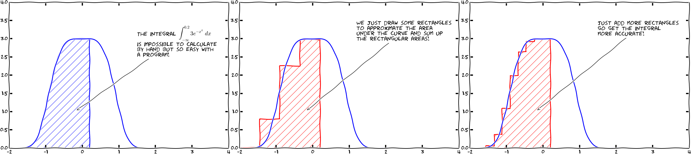
To understand and compare the numerical integration methods, it is advantageous to use a specific integral for computations and graphical illustrations. In particular, we want to use an integral that we can calculate by hand such that the accuracy of the approximation methods can easily be assessed. Our specific integral is taken from basic physics. Assume that you speed up your car from rest and wonder how far you go in \(T\) seconds. The distance is given by the integral \(\int_0^T v(t)dt\), where \(v(t)\) is the velocity as a function of time. A rapidly increasing velocity function might be

\[\tag{7} v\left(t\right) = 3t^{2}e^{t^3}\thinspace .\]

The distance after one second is

\[\tag{8} \int_0^1 v(t)dt,\]

which is the integral we aim to compute by numerical methods. Fortunately, the chosen expression of the velocity has a form that makes it easy to calculate the anti-derivative as

\[\tag{9} V(t) = e^{t^3}-1\thinspace .\]

We can therefore compute the exact value of the integral as \(V(1)-V(0)\approx 1.718\) (rounded to 3 decimals for convenience).

The composite trapezoidal rule

The integral \(\int_a^b f(x)dx\) may be interpreted as the area between the \(x\) axis and the graph \(y=f(x)\) of the integrand. Figure The integral of interpreted as the area under the graph of illustrates this area for the choice (8). Computing the integral \(\int_0^1f(t)dt\) amounts to computing the area of the hatched region.

The integral of \(v(t)\) interpreted as the area under the graph of \(v\)

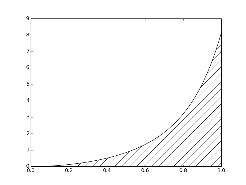
If we replace the true graph in Figure The integral of interpreted as the area under the graph of by a set of straight line segments, we may view the area rather as composed of trapezoids, the areas of which are easy to compute. This is illustrated in Figure Computing approximately the integral of a function as the sum of the areas of the trapezoids, where 4 straight line segments give rise to 4 trapezoids, covering the time intervals \([0,0.2)\), \([0.2,0.6)\), \([0.6,0.8)\) and \([0.8,1.0]\). Note that we have taken the opportunity here to demonstrate the computations with time intervals that differ in size.

Computing approximately the integral of a function as the sum of the areas of the trapezoids

The areas of the 4 trapezoids shown in Figure Computing approximately the integral of a function as the sum of the areas of the trapezoids now constitute our approximation to the integral (8):

\[\int_0^1 v(t)dt \approx h_1 (\frac{v(0)+v(0.2)}{2}) + h_2 (\frac{v(0.2)+v(0.6)}{2}) \nonumber\]

\[\tag{10} + h_3 (\frac{v(0.6)+v(0.8)}{2}) + h_4 (\frac{v(0.8)+v(1.0)}{2}),\]

where

\[\tag{11} h_1 = (0.2 - 0.0),\]

\[\tag{12} h_2 = (0.6 - 0.2),\]

\[\tag{13} h_3 = (0.8 - 0.6),\]

\[\tag{14} h_4 = (1.0 - 0.8)\thinspace\]

With \(v(t) = 3t^{2}e^{t^3}\), each term in (10) is readily computed and our approximate computation gives

\[\tag{15} \int_0^1 v(t)dt \approx 1.895\thinspace .\]

Compared to the true answer of \(1.718\), this is off by about 10%. However, note that we used just 4 trapezoids to approximate the area. With more trapezoids, the approximation would have become better, since the straight line segments in the upper trapezoid side then would follow the graph more closely. Doing another hand calculation with more trapezoids is not too tempting for a lazy human, though, but it is a perfect job for a computer! Let us therefore derive the expressions for approximating the integral by an arbitrary number of trapezoids.

For a given function \(f(x)\), we want to approximate the integral \(\int_a^bf(x)dx\) by \(n\) trapezoids (of equal width). We start out with (6) and approximate each integral on the right hand side with a single trapezoid. In detail,

\[\int_a^b f(x)\,dx = \int_{x_0}^{x_1} f(x) dx + \int_{x_1}^{x_2} f(x) dx + \ldots + \int_{x_{n-1}}^{x_n} f(x) dx, \nonumber\]

\[\approx h \frac{f(x_0) + f(x_1)}{2} + h \frac{f(x_1) + f(x_2)}{2} + \ldots + \nonumber\]

\[\tag{16} \quad h \frac{f(x_{n-1}) + f(x_n)}{2}\]

By simplifying the right hand side of (16) we get

\[\begin{split}\tag{17} \int_a^b f(x)\,dx \approx \\ \frac{h}{2}\left[f(x_0) + 2 f(x_1) + 2 f(x_2) + \ldots + 2 f(x_{n-1}) + f(x_n)\right]\end{split}\]

which is more compactly written as

\[\tag{18} \int_a^b f(x)\,dx \approx h \left[\frac{1}{2}f(x_0) + \sum_{i=1}^{n-1}f(x_i) + \frac{1}{2}f(x_n) \right] \thinspace .\]

Composite integration rules

The word composite is often used when a numerical integration method is applied with more than one sub-interval. Strictly speaking then, writing, e.g., “the trapezoidal method”, should imply the use of only a single trapezoid, while “the composite trapezoidal method” is the most correct name when several trapezoids are used. However, this naming convention is not always followed, so saying just “the trapezoidal method” may point to a single trapezoid as well as the composite rule with many trapezoids.

Specific or general implementation?

Suppose our primary goal was to compute the specific integral \(\int_0^1 v(t)dt\) with \(v(t)=3t^2e^{t^3}\). First we played around with a simple hand calculation to see what the method was about, before we (as one often does in mathematics) developed a general formula (18) for the general or “abstract” integral \(\int_a^bf(x)dx\). To solve our specific problem \(\int_0^1 v(t)dt\) we must then apply the general formula (18) to the given data (function and integral limits) in our problem. Although simple in principle, the practical steps are confusing for many because the notation in the abstract problem in (18) differs from the notation in our special problem. Clearly, the \(f\), \(x\), and \(h\) in (18) correspond to \(v\), \(t\), and perhaps \(\Delta t\) for the trapezoid width in our special problem.

The programmer’s dilemma

1. Should we write a special program for the special integral, using the ideas from the general rule (18), but replacing \(f\) by \(v\), \(x\) by \(t\), and \(h\) by \(\Delta t\)?
2. Should we implement the general method (18) as it stands in a general function trapezoid(f, a, b, n) and solve the specific problem at hand by a specialized call to this function?

Alternative 2 is always the best choice!

The first alternative in the box above sounds less abstract and therefore more attractive to many. Nevertheless, as we hope will be evident from the examples, the second alternative is actually the simplest and most reliable from both a mathematical and programming point of view. These authors will claim that the second alternative is the essence of the power of mathematics, while the first alternative is the source of much confusion about mathematics!

Implementation with functions

For the integral \(\int_a^bf(x)dx\) computed by the formula (18) we want the corresponding Python function trapezoid to take any \(f\), \(a\), \(b\), and \(n\) as input and return the approximation to the integral.

We write a Python function trapezoidal in a file trapezoidal.py as close as possible to the formula (18), making sure variable names correspond to the mathematical notation:

def trapezoidal(f, a, b, n):
    h = float(b-a)/n
    result = 0.5*f(a) + 0.5*f(b)
    for i in range(1, n):
        result += f(a + i*h)
    result *= h
    return result

Solving our specific problem in a session

Just having the trapezoidal function as the only content of a file trapezoidal.py automatically makes that file a module that we can import and test in an interactive session:

>>> from trapezoidal import trapezoidal
>>> from math import exp
>>> v = lambda t: 3*(t**2)*exp(t**3)
>>> n = 4
>>> numerical = trapezoidal(v, 0, 1, n)
>>> numerical
1.9227167504675762

Let us compute the exact expression and the error in the approximation:

>>> V = lambda t: exp(t**3)
>>> exact = V(1) - V(0)
>>> exact - numerical
-0.20443492200853108

Is this error convincing? We can try a larger \(n\):

>>> numerical = trapezoidal(v, 0, 1, n=400)
>>> exact - numerical
-2.1236490512777095e-05

Fortunately, many more trapezoids give a much smaller error.

Solving our specific problem in a program

Instead of computing our special problem in an interactive session, we can do it in a program. As always, a chunk of code doing a particular thing is best isolated as a function even if we do not see any future reason to call the function several times and even if we have no need for arguments to parameterize what goes on inside the function. In the present case, we just put the statements we otherwise would have put in a main program, inside a function:

def application():
    from math import exp
    v = lambda t: 3*(t**2)*exp(t**3)
    n = input('n: ')
    numerical = trapezoidal(v, 0, 1, n)

    # Compare with exact result
    V = lambda t: exp(t**3)
    exact = V(1) - V(0)
    error = exact - numerical
    print 'n=%d: %.16f, error: %g' % (n, numerical, error)

Now we compute our special problem by calling application() as the only statement in the main program. Both the trapezoidal and application functions reside in the file trapezoidal.py, which can be run as

Terminal> python trapezoidal.py
n: 4
n=4: 1.9227167504675762, error: -0.204435

Making a module

When we have the different pieces of our program as a collection of functions, it is very straightforward to create a module that can be imported in other programs. That is, having our code as a module, means that the trapezoidal function can easily be reused by other programs to solve other problems. The requirements of a module are simple: put everything inside functions and let function calls in the main program be in the so-called test block:

if __name__ == '__main__':
    application()

The if test is true if the module file, trapezoidal.py, is run as a program and false if the module is imported in another program. Consequently, when we do an import from trapezoidal import trapezoidal in some file, the test fails and application() is not called, i.e., our special problem is not solved and will not print anything on the screen. On the other hand, if we run trapezoidal.py in the terminal window, the test condition is positive, application() is called, and we get output in the window:

Terminal> python trapezoidal.py
n: 400
n=400: 1.7183030649495579, error: -2.12365e-05

Alternative flat special-purpose implementation

Let us illustrate the implementation implied by alternative 1 in the Programmer’s dilemma box in the section sec:integrals:trap:impl. That is, we make a special-purpose code where we adapt the general formula (18) to the specific problem \(\int_0^1 3t^2e^{t^3}dt\).

Basically, we use a for loop to compute the sum. Each term with \(f(x)\) in the formula (18) is replaced by \(3t^2e^{t^3}\), \(x\) by \(t\), and \(h\) by \(\Delta t\) [1]. A first try at writing a plain, flat program doing the special calculation is

from math import exp

a = 0.0;  b = 1.0
n = input('n: ')
dt = float(b - a)/n

# Integral by the trapezoidal method
numerical = 0.5*3*(a**2)*exp(a**3) + 0.5*3*(b**2)*exp(b**3)
for i in range(1, n):
    numerical += 3*((a + i*dt)**2)*exp((a + i*dt)**3)
numerical *= dt

exact_value = exp(1**3) - exp(0**3)
error = abs(exact_value - numerical)
rel_error = (error/exact_value)*100
print 'n=%d: %.16f, error: %g' % (n, numerical, error)

[1]	Replacing \(h\) by \(\Delta t\) is not strictly required as many use \(h\) as interval also along the time axis. Nevertheless, \(\Delta t\) is an even more popular notation for a small time interval, so we adopt that common notation.

The problem with the above code is at least three-fold:

1. We need to reformulate (18) for our special problem with a different notation.
2. The integrand \(3t^2e^{t^3}\) is inserted many times in the code, which quickly leads to errors.
3. A lot of edits are necessary to use the code to compute a different integral - these edits are likely to introduce errors.

The potential errors involved in point 2 serve to illustrate how important it is to use Python functions as mathematical functions. Here we have chosen to use the lambda function to define the integrand as the variable v:

from math import exp

v = lambda t: 3*(t**2)*exp(t**3)  # Function to be integrated
a = 0.0;  b = 1.0
n = input('n: ')
dt = float(b - a)/n

# Integral by the trapezoidal method
numerical = 0.5*v(a) + 0.5*v(b)
for i in range(1, n):
    numerical += v(a + i*dt)
numerical *= dt

F = lambda t: exp(t**3)
exact_value = F(b) - F(a)
error = abs(exact_value - numerical)
rel_error = (error/exact_value)*100
print 'n=%d: %.16f, error: %g' % (n, numerical, error)

Unfortunately, the two other problems remain and they are fundamental.

Suppose you want to compute another integral, say \(\int_{-1}^{1.1}e^{-x^2}dx\). How much do we need to change in the previous code to compute the new integral? Not so much:

• the formula for v must be replaced by a new formula
• the limits a and b
• the anti-derivative \(V\) is not easily known [2] and can be omitted, and therefore we cannot write out the error
• the notation should be changed to be aligned with the new problem, i.e., t and dt changed to x and h

[2]	You cannot integrate \(e^{-x^2}\) by hand, but this particular integral is appearing so often in so many contexts that the integral is a special function, called the Error function and written \(\mbox{erf}(x)\). In a code, you can call erf(x). The erf function is found in the math module.

These changes are straightforward to implement, but they are scattered around in the program, a fact that requires us to be very careful so we do not introduce new programming errors while we modify the code. It is also very easy to forget to make a required change.

With the previous code in trapezoidal.py, we can compute the new integral \(\int_{-1}^{1.1}e^{-x^2}dx\) without touching the mathematical algorithm. In an interactive session (or in a program) we can just do

>>> from trapezoidal import trapezoidal
>>> from math import exp
>>> trapezoidal(lambda x: exp(-x**2), -1, 1.1, 400)
1.5268823686123285

When you now look back at the two solutions, the flat special-purpose program and the function-based program with the general-purpose function trapezoidal, you hopefully realize that implementing a general mathematical algorithm in a general function requires somewhat more abstract thinking, but the resulting code can be used over and over again. Essentially, if you apply the flat special-purpose style, you have to retest the implementation of the algorithm after every change of the program.

The present integral problems result in short code. In more challenging engineering problems the code quickly grows to hundreds and thousands of line. Without abstractions in terms of general algorithms in general reusable functions, the complexity of the program grows so fast that it will be extremely difficult to make sure that the program works properly.

Another advantage of packaging mathematical algorithms in functions is that a function can be reused by anyone to solve a problem by just calling the function with a proper set of arguments. Understanding the function’s inner details is not necessary to compute a new integral. Similarly, you can find libraries of functions on the Internet and use these functions to solve your problems without specific knowledge of every mathematical detail in the functions.

This desirable feature has its downside, of course: the user of a function may misuse it, and the function may contain programming errors and lead to wrong answers. Testing the output of downloaded functions is therefore extremely important before relying on the results.

The composite midpoint method

The idea

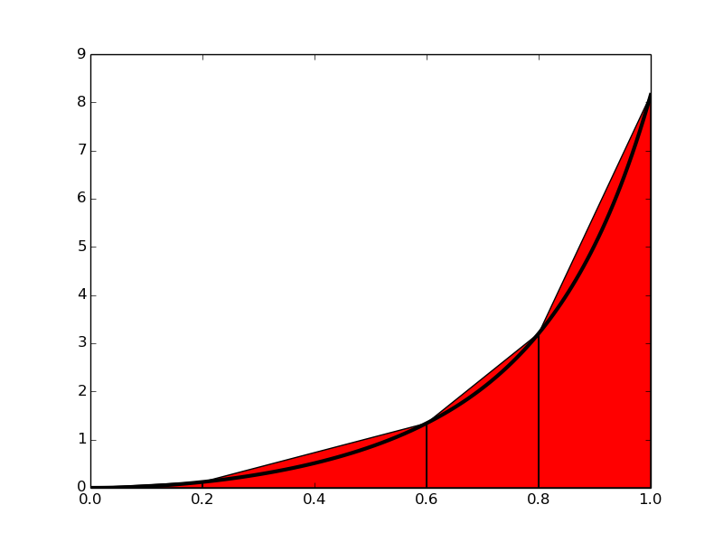
Rather than approximating the area under a curve by trapezoids, we can use plain rectangles. It may sound less accurate to use horizontal lines and not skew lines following the function to be integrated, but an integration method based on rectangles (the midpoint method) is in fact slightly more accurate than the one based on trapezoids!

In the midpoint method, we construct a rectangle for every sub-interval where the height equals \(f\) at the midpoint of the sub-interval. Let us do this for four rectangles, using the same sub-intervals as we had for hand calculations with the trapezoidal method: \([0,0.2)\), \([0.2,0.6)\), \([0.6,0.8)\), and \([0.8,1.0]\). We get

\[\int_0^1 f(t)dt \approx h_1 f\left(\frac{0 + 0.2}{2}\right) + h_2 f\left(\frac{0.2 + 0.6}{2}\right) \nonumber\]

\[\tag{19} + h_3 f\left(\frac{0.6 + 0.8}{2}\right) + h_4 f\left(\frac{0.8 + 1.0}{2}\right),\]

where \(h_1\), \(h_2\), \(h_3\), and \(h_4\) are the widths of the sub-intervals, used previously with the trapezoidal method and defined in (11)-(14).

Computing approximately the integral of a function as the sum of the areas of the rectangles

With \(f(t) = 3t^{2}e^{t^3}\), the approximation becomes \(1.632\). Compared with the true answer (\(1.718\)), this is about \(5\%\) too small, but it is better than what we got with the trapezoidal method (\(10\%\)) with the same sub-intervals. More rectangles give a better approximation.

The general formula

Let us derive a formula for the midpoint method based on \(n\) rectangles of equal width:

\[\int_a^b f(x)\,dx = \int_{x_0}^{x_1} f(x)dx + \int_{x_1}^{x_2} f(x)dx + \ldots + \int_{x_{n-1}}^{x_n} f(x)dx, \nonumber\]

\[\tag{20} \approx h f\left(\frac{x_0 + x_1}{2}\right) + h f\left(\frac{x_1 + x_2}{2}\right) + \ldots + h f\left(\frac{x_{n-1} + x_n}{2}\right) ,\]

\[\tag{21} \approx h \left(f\left(\frac{x_0 + x_1}{2}\right) + f\left(\frac{x_1 + x_2}{2}\right) + \ldots + f\left(\frac{x_{n-1} + x_n}{2}\right)\right)\thinspace .\]

This sum may be written more compactly as

\[\tag{22} \int_a^b f(x) dx \approx h \sum_{i=0}^{n-1}f(x_i) ,\]

where \(x_i = \left(a + \frac{h}{2}\right) + ih\).

Implementation

We follow the advice and lessons learned from the implementation of the trapezoidal method and make a function midpoint(f, a, b, n) (in a file midpoint.py) for implementing the general formula (22):

def midpoint(f, a, b, n):
    h = float(b-a)/n
    result = 0
    for i in range(n):
        result += f((a + h/2.0) + i*h)
    result *= h
    return result

We can test the function as we explained for the similar trapezoidal method. The error in our particular problem \(\int_0^1 3t^2e^{t^3}dt\) with four intervals is now about 0.1 in contrast to 0.2 for the trapezoidal rule. This is in fact not accidental: one can show mathematically that the error of the midpoint method is a bit smaller than for the trapezoidal method. The differences are seldom of any practical importance, and on a laptop we can easily use \(n=10^6\) and get the answer with an error about \(10^{-12}\) in a couple of seconds.

Comparing the trapezoidal and the midpoint methods

The next example shows how easy we can combine the trapezoidal and midpoint functions to make a comparison of the two methods in the file compare_integration_methods.py:

from trapezoidal import trapezoidal
from midpoint import midpoint
from math import exp

g = lambda y: exp(-y**2)
a = 0
b = 2
print '    n        midpoint          trapezoidal'
for i in range(1, 21):
    n = 2**i
    m = midpoint(g, a, b, n)
    t = trapezoidal(g, a, b, n)
    print '%7d %.16f %.16f' % (n, m, t)

Note the efforts put into nice formatting - the output becomes

    n        midpoint          trapezoidal
      2 0.8842000076332692 0.8770372606158094
      4 0.8827889485397279 0.8806186341245393
      8 0.8822686991994210 0.8817037913321336
     16 0.8821288703366458 0.8819862452657772
     32 0.8820933014203766 0.8820575578012112
     64 0.8820843709743319 0.8820754296107942
    128 0.8820821359746071 0.8820799002925637
    256 0.8820815770754198 0.8820810181335849
    512 0.8820814373412922 0.8820812976045025
   1024 0.8820814024071774 0.8820813674728968
   2048 0.8820813936736116 0.8820813849400392
   4096 0.8820813914902204 0.8820813893068272
   8192 0.8820813909443684 0.8820813903985197
  16384 0.8820813908079066 0.8820813906714446
  32768 0.8820813907737911 0.8820813907396778
  65536 0.8820813907652575 0.8820813907567422
 131072 0.8820813907631487 0.8820813907610036
 262144 0.8820813907625702 0.8820813907620528
 524288 0.8820813907624605 0.8820813907623183
1048576 0.8820813907624268 0.8820813907623890

A visual inspection of the numbers shows how fast the digits stabilize in both methods. It appears that 13 digits have stabilized in the last two rows.

Remark

The trapezoidal and midpoint methods are just two examples in a jungle of numerical integration rules. Other famous methods are Simpson’s rule and Gauss quadrature. They all work in the same way:

\[\int_a^b f(x)dx \approx \sum_{i=0}^{n-1} w_if(x_i)\thinspace .\]

That is, the integral is approximated by a sum of function evaluations, where each evaluation \(f(x_i)\) is given a weight \(w_i\). The different methods differ in the way they construct the evaluation points \(x_i\) and the weights \(w_i\). We have used equally spaced points \(x_i\), but higher accuracy can be obtained by optimizing the location of \(x_i\).

Testing

Testing of the programs for numerical integration has so far employed two strategies. If we have an exact answer, we compute the error and see that increasing \(n\) decreases the error. When the exact answer is not available, we can (as in the comparison example in the previous section) look at the integral values and see that they stabilize as \(n\) grows. Unfortunately, these are very weak test procedures and not at all satisfactory for claiming that the software we have produced is correctly implemented.

To see this, we can introduce a bug in the application function that calls trapezoidal: instead of integrating \(3t^2e^{t^3}\), we write “accidentally” \(3t^3e^{t^3}\), but keep the same anti-derivative \(V(t)e^{t^3}\) for computing the error. With the bug and \(n=4\), the error is 0.1, but without the bug the error is 0.2! It is of course completely impossible to tell if 0.1 is the right value of the error. Fortunately, increasing \(n\) shows that the error stays about 0.3 in the program with the bug, so the test procedure with increasing \(n\) and checking that the error decreases points to a problem in the code.

Let us look at another bug, this time in the mathematical algorithm: instead of computing \(\frac{1}{2}(f(a) + f(b))\) as we should, we forget the second \(\frac{1}{2}\) and write 0.5*f(a) + f(b). The error for \(n=4,40,400\) when computing \(\int_{1.1}^{1.9} 3t^2e^{t^3}dt\) goes like \(1400\), \(107\), \(10\), respectively, which looks promising. The problem is that the right errors should be \(369\), \(4.08\), and \(0.04\). That is, the error should be reduced faster in the correct than in the buggy code. The problem, however, is that it is reduced in both codes, and we may stop further testing and believe everything is correctly implemented.

Unit testing

A good habit is to test small pieces of a larger code individually, one at a time. This is known as unit testing. One identifies a (small) unit of the code, and then one makes a separate test for this unit. The unit test should be stand-alone in the sense that it can be run without the outcome of other tests. Typically, one algorithm in scientific programs is considered as a unit. The challenge with unit tests in numerical computing is to deal with numerical approximation errors. A fortunate side effect of unit testing is that the programmer is forced to use functions to modularize the code into smaller, logical pieces.

There are three serious ways to test the implementation of numerical methods via unit tests:

1. Comparing with hand-computed results in a problem with few arithmetic operations, i.e., small \(n\).
2. Solving a problem without numerical errors. We know that the trapezoidal rule must be exact for linear functions. The error produced by the program must then be zero (to machine precision).
3. Demonstrating correct convergence rates. A strong test when we can compute exact errors, is to see how fast the error goes to zero as \(n\) grows. In the trapezoidal and midpoint rules it is known that the error depends on \(n\) as \(n^{-2}\) as \(n\rightarrow\infty\).

Hand-computed results

Let us use two trapezoids and compute the integral \(\int_0^1v(t)\), \(v(t)=3t^2e^{t^3}\):

\[\frac{1}{2}h(v(0) + v(0.5)) + \frac{1}{2}h(v(0.5)+v(1)) = 2.463642041244344,\]

when \(h=0.5\) is the width of the two trapezoids. Running the program gives exactly the same results.

Solving a problem without numerical errors

The best unit tests for numerical algorithms involve mathematical problems where we know the numerical result beforehand. Usually, numerical results contain unknown approximation errors, so knowing the numerical result implies that we have a problem where the approximation errors vanish. This feature may be present in very simple mathematical problems. For example, the trapezoidal method is exact for integration of linear functions \(f(x)=ax+b\). We can therefore pick some linear function and construct a test function that checks equality between the exact analytical expression for the integral and the number computed by the implementation of the trapezoidal method.

A specific test case can be \(\int_{1.2}^{4.4} (6x-4)dx\). This integral involves an “arbitrary” interval \([1.2, 4.4]\) and an “arbitrary” linear function \(f(x) = 6x-4\). By “arbitrary” we mean expressions where we avoid the special numbers 0 and 1 since these have special properties in arithmetic operations (e.g., forgetting to multiply is equivalent to multiplying by 1, and forgetting to add is equivalent to adding 0).

Demonstrating correct convergence rates

Normally, unit tests must be based on problems where the numerical approximation errors in our implementation remain unknown. However, we often know or may assume a certain asymptotic behavior of the error. We can do some experimental runs with the test problem \(\int_0^1 3t^2e^{t^3}dt\) where \(n\) is doubled in each run: \(n=4,8,16\). The corresponding errors are then 12%, 3% and 0.77%, respectively. These numbers indicate that the error is roughly reduced by a factor of 4 when doubling \(n\). Thus, the error converges to zero as \(n^{-2}\) and we say that the convergence rate is 2. In fact, this result can also be shown mathematically for the trapezoidal and midpoint method. Numerical integration methods usually have an error that converge to zero as \(n^{-p}\) for some \(p\) that depends on the method. With such a result, it does not matter if we do not know what the actual approximation error is: we know at what rate it is reduced, so running the implementation for two or more different \(n\) values will put us in a position to measure the expected rate and see if it is achieved.

The idea of a corresponding unit test is then to run the algorithm for some \(n\) values, compute the error (the absolute value of the difference between the exact analytical result and the one produced by the numerical method), and check that the error has approximately correct asymptotic behavior, i.e., that the error is proportional to \(n^{-2}\) in case of the trapezoidal and midpoint method.

Let us develop a more precise method for such unit tests based on convergence rates. We assume that the error \(E\) depends on \(n\) according to

\[E = Cn^r,\]

where \(C\) is an unknown constant and \(r\) is the convergence rate. Consider a set of experiments with various \(n\): \(n_0, n_1, n_2, \ldots,n_q\). We compute the corresponding errors \(E_0,\ldots,E_q\). For two consecutive experiments, number \(i\) and \(i-1\), we have the error model

\[\tag{23} E_{i} = Cn_{i}^r,\]

\[\tag{24} E_{i-1} = Cn_{i-1}^r\thinspace .\]

These are two equations for two unknowns \(C\) and \(r\). We can easily eliminate \(C\) by dividing the equations by each other. Then solving for \(r\) gives

\[\tag{25} r_{i-1} = \frac{\ln (E_i/E_{i-1})}{\ln (n_i/n_{i-1})}\thinspace .\]

We have introduced a subscript \(i-1\) in \(r\) since the estimated value for \(r\) varies with \(i\). Hopefully, \(r_{i-1}\) approaches the correct convergence rate as the number of intervals increases and \(i\rightarrow q\).

Finite precision of floating-point numbers

The test procedures above lead to comparison of numbers for checking that calculations were correct. Such comparison is more complicated than what a newcomer might think. Suppose we have a calculation a + b and want to check that the result is what we expect. We start with 1 + 2:

>>> a = 1; b = 2; expected = 3
>>> a + b == expected
True

Then we proceed with 0.1 + 0.2:

>>> a = 0.1; b = 0.2; expected = 0.3
>>> a + b == expected
False

So why is \(0.1 + 0.2 \neq 0.3\)? The reason is that real numbers cannot in general be exactly represented on a computer. They must instead be approximated by a floating-point number that can only store a finite amount of information, usually about 17 digits of a real number. Let us print 0.1, 0.2, 0.1 + 0.2, and 0.3 with 17 decimals:

>>> print '%.17f\n%.17f\n%.17f\n%.17f' % (0.1, 0.2, 0.1 + 0.2, 0.3)
0.10000000000000001
0.20000000000000001
0.30000000000000004
0.29999999999999999

We see that all of the numbers have an inaccurate digit in the 17th decimal place. Because 0.1 + 0.2 evaluates to 0.30000000000000004 and 0.3 is represented as 0.29999999999999999, these two numbers are not equal. In general, real numbers in Python have (at most) 16 correct decimals.

When we compute with real numbers, these numbers are inaccurately represented on the computer, and arithmetic operations with inaccurate numbers lead to small rounding errors in the final results. Depending on the type of numerical algorithm, the rounding errors may or may not accumulate.

If we cannot make tests like 0.1 + 0.2 == 0.3, what should we then do? The answer is that we must accept some small inaccuracy and make a test with a tolerance. Here is the recipe:

>>> a = 0.1; b = 0.2; expected = 0.3
>>> computed = a + b
>>> diff = abs(expected - computed)
>>> tol = 1E-15
>>> diff < tol
True

Here we have set the tolerance for comparison to \(10^{-15}\), but calculating 0.3 - (0.1 + 0.2) shows that it equals -5.55e-17, so a lower tolerance could be used in this particular example. However, in other calculations we have little idea about how accurate the answer is (there could be accumulation of rounding errors in more complicated algorithms), so \(10^{-15}\) or \(10^{-14}\) are robust values. As we demonstrate below, these tolerances depend on the magnitude of the numbers in the calculations.

Doing an experiment with \(10^k + 0.3 - (10^k + 0.1 + 0.2)\) for \(k=1,\ldots,10\) shows that the answer (which should be zero) is around \(10^{16-k}\). This means that the tolerance must be larger if we compute with larger numbers. Setting a proper tolerance therefore requires some experiments to see what level of accuracy one can expect. A way out of this difficulty is to work with relative instead of absolute differences. In a relative difference we divide by one of the operands, e.g.,

\[a = 10^k + 0.3,\quad b = (10^k + 0.1 + 0.2),\quad c = \frac{a - b}{a}\thinspace .\]

Computing this \(c\) for various \(k\) shows a value around \(10^{-16}\). A safer procedure is thus to use relative differences.

Constructing unit tests and writing test functions

Python has several frameworks for automatically running and checking a potentially very large number of tests for parts of your software by one command. This is an extremely useful feature during program development: whenever you have done some changes to one or more files, launch the test command and make sure nothing is broken because of your edits.

The test frameworks nose and py.test are particularly attractive as they are very easy to use. Tests are placed in special test functions that the frameworks can recognize and run for you. The requirements to a test function are simple:

• the name must start with test_
• the test function cannot have any arguments
• the tests inside test functions must be boolean expressions
• a boolean expression b must be tested with assert b, msg, where msg is an optional object (string or number) to be written out when b is false

Suppose we have written a function

def add(a, b):
    return a + b

A corresponding test function can then be

def test_add()
    expected = 1 + 1
    computed = add(1, 1)
    assert computed == expected, '1+1=%g' % computed

Test functions can be in any program file or in separate files, typically with names starting with test. You can also collect tests in subdirectories: running py.test -s -v will actually run all tests in all test*.py files in all subdirectories, while nosetests -s -v restricts the attention to subdirectories whose names start with test or end with _test or _tests.

As long as we add integers, the equality test in the test_add function is appropriate, but if we try to call add(0.1, 0.2) instead, we will face the rounding error problems explained in the section Finite precision of floating-point numbers, and we must use a test with tolerance instead:

def test_add()
    expected = 0.3
    computed = add(0.1, 0.2)
    tol = 1E-14
    diff = abs(expected - computed)
    assert diff < tol, 'diff=%g' % diff

Below we shall write test functions for each of the three test procedures we suggested: comparison with hand calculations, checking problems that can be exactly solved, and checking convergence rates. We stick to testing the trapezoidal integration code and collect all test functions in one common file by the name test_trapezoidal.py.

Hand-computed numerical results

Our previous hand calculations for two trapezoids can be checked against the trapezoidal function inside a test function (in a file test_trapezoidal.py):

from trapezoidal import trapezoidal

def test_trapezoidal_one_exact_result():
    """Compare one hand-computed result."""
    from math import exp
    v = lambda t: 3*(t**2)*exp(t**3)
    n = 2
    computed = trapezoidal(v, 0, 1, n)
    expected = 2.463642041244344
    error = abs(expected - computed)
    tol = 1E-14
    success = error < tol
    msg = 'error=%g > tol=%g' % (errror, tol)
    assert success, msg

Note the importance of checking err against exact with a tolerance: rounding errors from the arithmetics inside trapezoidal will not make the result exactly like the hand-computed one. The size of the tolerance is here set to \(10^{-14}\), which is a kind of all-round value for computations with numbers not deviating much from unity.

Solving a problem without numerical errors

We know that the trapezoidal rule is exact for linear integrands. Choosing the integral \(\int_{1.2}^{4.4} (6x-4)dx\) as test case, the corresponding test function for this unit test may look like

def test_trapezoidal_linear():
    """Check that linear functions are integrated exactly."""
    f = lambda x: 6*x - 4
    F = lambda x: 3*x**2 - 4*x  # Anti-derivative
    a = 1.2; b = 4.4
    expected = F(b) - F(a)
    tol = 1E-14
    for n in 2, 20, 21:
        computed = trapezoidal(f, a, b, n)
        error = abs(expected - computed)
        success = error < tol
        msg = 'n=%d, err=%g' % (n, error)
        assert success, msg

Demonstrating correct convergence rates

In the present example with integration, it is known that the approximation errors in the trapezoidal rule are proportional to \(n^{-2}\), \(n\) being the number of subintervals used in the composite rule.

Computing convergence rates requires somewhat more tedious programming than the previous tests, but can be applied to more general integrands. The algorithm typically goes like

• for \(i=0,1,2,\ldots,q\)
  • \(n_i = 2^{i+1}\)
  • Compute integral with \(n_i\) intervals
  • Compute the error \(E_i\)
  • Estimate \(r_i\) from (25) if \(i>0\)

The corresponding code may look like

def convergence_rates(f, F, a, b, num_experiments=14):
    from math import log
    from numpy import zeros
    expected = F(b) - F(a)
    n = zeros(num_experiments, dtype=int)
    E = zeros(num_experiments)
    r = zeros(num_experiments-1)
    for i in range(num_experiments):
        n[i] = 2**(i+1)
        computed = trapezoidal(f, a, b, n[i])
        E[i] = abs(expected - computed)
        if i > 0:
            r_im1 = log(E[i]/E[i-1])/log(float(n[i])/n[i-1])
            r[i-1] = float('%.2f' % r_im1) # Truncate to two decimals
    return r

Making a test function is a matter of choosing f, F, a, and b, and then checking the value of \(r_i\) for the largest \(i\):

def test_trapezoidal_conv_rate():
    """Check empirical convergence rates against the expected -2."""
    from math import exp
    v = lambda t: 3*(t**2)*exp(t**3)
    V = lambda t: exp(t**3)
    a = 1.1; b = 1.9
    r = convergence_rates(v, V, a, b, 14)
    print r
    tol = 0.01
    msg = str(r[-4:])  # show last 4 estimated rates
    assert (abs(r[-1]) - 2) < tol, msg

Running the test shows that all \(r_i\), except the first one, equal the target limit 2 within two decimals. This observation suggest a tolerance of \(10^{-2}\).

Remark about version control of files

Having a suite of test functions for automatically checking that your software works is considered as a fundamental requirement for reliable computing. Equally important is a system that can keep track of different versions of the files and the tests, known as a version control system. Today’s most popular version control system is Git, which the authors strongly recommend the reader to use for programming and writing reports. The combination of Git and cloud storage such as GitHub is a very common way of organizing scientific or engineering work. We have a quick intro to Git and GitHub that gets you up and running within minutes.

The typical workflow with Git goes as follows.

1. Before you start working with files, make sure you have the latest version of them by running git pull.
2. Edit files, remove or create files (new files must be registered by git add).
3. When a natural piece of work is done, commit your changes by the git commit command.
4. Implement your changes also in the cloud by doing git push.

A nice feature of Git is that people can edit the same file at the same time and very often Git will be able to automatically merge the changes (!). Therefore, version control is crucial when you work with others or when you do your work on different types of computers. Another key feature is that anyone can at any time view the history of a file, see who did what when, and roll back the entire file collection to a previous commit. This feature is, of course, fundamental for reliable work.

Vectorization

The functions midpoint and trapezoid usually run fast in Python and compute an integral to a satisfactory precision within a fraction of a second. However, long loops in Python may run slowly in more complicated implementations. To increase the speed, the loops can be replaced by vectorized code. The integration functions constitute a simple and good example to illustrate how to vectorize loops.

We have already seen simple examples on vectorization in the section A Python program with vectorization and plotting when we could evaluate a mathematical function \(f(x)\) for a large number of \(x\) values stored in an array. Basically, we can write

def f(x):
    return exp(-x)*sin(x) + 5*x

from numpy import exp, sin, linspace
x = linspace(0, 4, 101)  # coordinates from 100 intervals on [0, 4]
y = f(x)                 # all points evaluated at once

The result y is the array that would be computed if we ran a for loop over the individual x values and called f for each value. Vectorization essentially eliminates this loop in Python (i.e., the looping over x and application of f to each x value are instead performed in a library with fast, compiled code).

Vectorizing the midpoint rule

The aim of vectorizing the midpoint and trapezoidal functions is also to remove the explicit loop in Python. We start with vectorizing the midpoint function since trapezoid is not equally straightforward. The fundamental ideas of the vectorized algorithm are to

1. compute all the evaluation points in one array x
2. call f(x) to produce an array of corresponding function values
3. use the sum function to sum the f(x) values

The evaluation points in the midpoint method are \(x_i=a+(i+\frac{1}{2})h\), \(i=0,\ldots,n-1\). That is, \(n\) uniformly distributed coordinates between \(a+h/2\) and \(b-h/2\). Such coordinates can be calculated by x = linspace(a+h/2, b-h/2, n). Given that the Python implementation f of the mathematical function \(f\) works with an array argument, which is very often the case in Python, f(x) will produce all the function values in an array. The array elements are then summed up by sum: sum(f(x)). This sum is to be multiplied by the rectangle width \(h\) to produce the integral value. The complete function is listed below.

from numpy import linspace, sum

def midpoint(f, a, b, n):
    h = float(b-a)/n
    x = linspace(a + h/2, b - h/2, n)
    return h*sum(f(x))

The code is found in the file integration_methods_vec.py.

Let us test the code interactively in a Python shell to compute \(\int_0^1 3t^2dt\). The file with the code above has the name integration_methods_vec.py and is a valid module from which we can import the vectorized function:

>>> from integration_methods_vec import midpoint
>>> from numpy import exp
>>> v = lambda t: 3*t**2*exp(t**3)
>>> midpoint(v, 0, 1, 10)
1.7014827690091872

Note the necessity to use exp from numpy: our v function will be called with x as an array, and the exp function must be capable of working with an array.

The vectorized code performs all loops very efficiently in compiled code, resulting in much faster execution. Moreover, many readers of the code will also say that the algorithm looks clearer than in the loop-based implementation.

Vectorizing the trapezoidal rule

We can use the same approach to vectorize the trapezoid function. However, the trapezoidal rule performs a sum where the end points have different weight. If we do sum(f(x)), we get the end points f(a) and f(b) with weight unity instead of one half. A remedy is to subtract the error from sum(f(x)): sum(f(x)) - 0.5*f(a) - 0.5*f(b). The vectorized version of the trapezoidal method then becomes

def trapezoidal(f, a, b, n):
    h = float(b-a)/n
    x = linspace(a, b, n+1)
    s = sum(f(x)) - 0.5*f(a) - 0.5*f(b)
    return h*s

Measuring computational speed

Now that we have created faster, vectorized versions of functions in the previous section, it is interesting to measure how much faster they are. The purpose of the present section is therefore to explain how we can record the CPU time consumed by a function so we can answer this question. There are many techniques for measuring the CPU time in Python, and here we shall just explain the simplest and most convenient one: the %timeit command in IPython. The following interactive session should illustrate a competition where the vectorized versions of the functions are supposed to win:

In [1]: from integration_methods_vec import midpoint as midpoint_vec

In [3]: from midpoint import midpoint

In [4]: from numpy import exp

In [5]: v = lambda t: 3*t**2*exp(t**3)

In [6]: %timeit midpoint_vec(v, 0, 1, 1000000)
1 loops, best of 3: 379 ms per loop

In [7]: %timeit midpoint(v, 0, 1, 1000000)
1 loops, best of 3: 8.17 s per loop

In [8]: 8.17/(379*0.001)    # efficiency factor
Out[8]: 21.556728232189972

We see that the vectorized version is about 20 times faster: 379 ms versus 8.17 s. The results for the trapezoidal method are very similar, and the factor of about 20 is independent of the number of intervals.

Double and triple integrals

Given a double integral over a rectangular domain \([a,b]\times [c,d]\),

\[\int_a^b \int_c^d f(x,y) dydx,\]

how can we approximate this integral by numerical methods?

Derivation via one-dimensional integrals

Since we know how to deal with integrals in one variable, a fruitful approach is to view the double integral as two integrals, each in one variable, which can be approximated numerically by previous one-dimensional formulas. To this end, we introduce a help function \(g(x)\) and write

\[\int_a^b \int_c^d f(x,y) dydx = \int_a^b g(x)dx,\quad g(x) = \int_c^d f(x,y) dy\thinspace .\]

Each of the integrals

\[\int_a^b g(x)dx,\quad g(x) = \int_c^d f(x,y) dy\]

can be discretized by any numerical integration rule for an integral in one variable. Let us use the midpoint method (22) and start with \(g(x)=\int_c^d f(x,y)dy\). We introduce \(n_y\) intervals on \([c,d]\) with length \(h_y\). The midpoint rule for this integral then becomes

\[g(x) = \int_c^d f(x,y) dy \approx h_y \sum_{j=0}^{n_y-1} f(x,y_j), \quad y_j = c + \frac{1}{2}{h_y} + jh_y \thinspace .\]

The expression looks somewhat different from (22), but that is because of the notation: since we integrate in the \(y\) direction and will have to work with both \(x\) and \(y\) as coordinates, we must use \(n_y\) for \(n\), \(h_y\) for \(h\), and the counter \(i\) is more naturally called \(j\) when integrating in \(y\). Integrals in the \(x\) direction will use \(h_x\) and \(n_x\) for \(h\) and \(n\), and \(i\) as counter.

The double integral is \(\int_a^b g(x)dx\), which can be approximated by the midpoint method:

\[\int_a^b g(x)dx \approx h_x \sum_{i=0}^{n_x-1} g(x_i),\quad x_i=a + \frac{1}{2}{h_x} + ih_x\thinspace .\]

Putting the formulas together, we arrive at the composite midpoint method for a double integral:

\[\int_a^b \int_c^d f(x,y) dydx \approx h_x \sum_{i=0}^{n_x-1} h_y \sum_{j=0}^{n_y-1} f(x_i,y_j)\nonumber\]

\[\tag{26} = h_xh_y \sum_{i=0}^{n_x-1} \sum_{j=0}^{n_y-1} f(a + \frac{h_x}{2} + ih_x, c + \frac{h_y}{2} + jh_y)\thinspace .\]

Direct derivation

The formula (26) can also be derived directly in the two-dimensional case by applying the idea of the midpoint method. We divide the rectangle \([a,b]\times [c,d]\) into \(n_x\times n_y\) equal-sized cells. The idea of the midpoint method is to approximate \(f\) by a constant over each cell, and evaluate the constant at the midpoint. Cell \((i,j)\) occupies the area

\[[a+ih_x,a+(i+1)h_x]\times [c+jh_y, c+ (j+1)h_y],\]

and the midpoint is \((x_i,y_j)\) with

\[x_i=a + ih_x + \frac{1}{2}{h_x} ,\quad y_j = c + jh_y + \frac{1}{2}{h_y} \thinspace .\]

The integral over the cell is therefore \(h_xh_y f(x_i,y_j)\), and the total double integral is the sum over all cells, which is nothing but formula (26).

Programming a double sum

The formula (26) involves a double sum, which is normally implemented as a double for loop. A Python function implementing (26) may look like

def midpoint_double1(f, a, b, c, d, nx, ny):
    hx = (b - a)/float(nx)
    hy = (d - c)/float(ny)
    I = 0
    for i in range(nx):
        for j in range(ny):
            xi = a + hx/2 + i*hx
            yj = c + hy/2 + j*hy
            I += hx*hy*f(xi, yj)
    return I

If this function is stored in a module file midpoint_double.py, we can compute some integral, e.g., \(\int_2^3\int_0^2 (2x + y)dxdy=9\) in an interactive shell and demonstrate that the function computes the right number:

>>> from midpoint_double import midpoint_double1
>>> def f(x, y):
...     return 2*x + y
...
>>> midpoint_double1(f, 0, 2, 2, 3, 5, 5)
9.0

Reusing code for one-dimensional integrals

It is very natural to write a two-dimensional midpoint method as we did in function midpoint_double1 when we have the formula (26). However, we could alternatively ask, much as we did in the mathematics, can we reuse a well-tested implementation for one-dimensional integrals to compute double integrals? That is, can we use function midpoint

def midpoint(f, a, b, n):
    h = float(b-a)/n
    result = 0
    for i in range(n):
        result += f((a + h/2.0) + i*h)
    result *= h
    return result

from the section Implementation “twice”? The answer is yes, if we think as we did in the mathematics: compute the double integral as a midpoint rule for integrating \(g(x)\) and define \(g(x_i)\) in terms of a midpoint rule over \(f\) in the \(y\) coordinate. The corresponding function has very short code:

def midpoint_double2(f, a, b, c, d, nx, ny):
    def g(x):
        return midpoint(lambda y: f(x, y), c, d, ny)

    return midpoint(g, a, b, nx)

The important advantage of this implementation is that we reuse a well-tested function for the standard one-dimensional midpoint rule and that we apply the one-dimensional rule exactly as in the mathematics.

Verification via test functions

How can we test that our functions for the double integral work? The best unit test is to find a problem where the numerical approximation error vanishes because then we know exactly what the numerical answer should be. The midpoint rule is exact for linear functions, regardless of how many subinterval we use. Also, any linear two-dimensional function \(f(x,y)=px+qy+r\) will be integrated exactly by the two-dimensional midpoint rule. We may pick \(f(x,y)=2x+y\) and create a proper test function that can automatically verify our two alternative implementations of the two-dimensional midpoint rule. To compute the integral of \(f(x,y)\) we take advantage of SymPy to eliminate the possibility of errors in hand calculations. The test function becomes

def test_midpoint_double():
    """Test that a linear function is integrated exactly."""
    def f(x, y):
        return 2*x + y

    a = 0;  b = 2;  c = 2;  d = 3
    import sympy
    x, y = sympy.symbols('x  y')
    I_expected = sympy.integrate(f(x, y), (x, a, b), (y, c, d))
    # Test three cases: nx < ny, nx = ny, nx > ny
    for nx, ny in (3, 5), (4, 4), (5, 3):
        I_computed1 = midpoint_double1(f, a, b, c, d, nx, ny)
        I_computed2 = midpoint_double2(f, a, b, c, d, nx, ny)
        tol = 1E-14
        #print I_expected, I_computed1, I_computed2
        assert abs(I_computed1 - I_expected) < tol
        assert abs(I_computed2 - I_expected) < tol

Let test functions speak up

If we call the above test_midpoint_double function and nothing happens, our implementations are correct. However, it is somewhat annoying to have a function that is completely silent when it works - are we sure all things are properly computed? During development it is therefore highly recommended to insert a print statement such that we can monitor the calculations and be convinced that the test function does what we want. Since a test function should not have any print statement, we simply comment it out as we have done in the function listed above.

The trapezoidal method can be used as alternative for the midpoint method. The derivation of a formula for the double integral and the implementations follow exactly the same ideas as we explained with the midpoint method, but there are more terms to write in the formulas. Exercise 42: Derive the trapezoidal rule for a double integral asks you to carry out the details. That exercise is a very good test on your understanding of the mathematical and programming ideas in the present section.

The midpoint rule for a triple integral

Theory

Once a method that works for a one-dimensional problem is generalized to two dimensions, it is usually quite straightforward to extend the method to three dimensions. This will now be demonstrated for integrals. We have the triple integral

\[\int_{a}^{b} \int_c^d \int_e^f g(x,y,z) dzdydx\]

and want to approximate the integral by a midpoint rule. Following the ideas for the double integral, we split this integral into one-dimensional integrals:

\[\begin{split}p(x,y) &= \int_e^f g(x,y,z) dz\\ q(x) &= \int_c^d p(x,y) dy\\ \int_{a}^{b} \int_c^d \int_e^f g(x,y,z) dzdydx &= \int_a^b q(x)dx\end{split}\]

For each of these one-dimensional integrals we apply the midpoint rule:

\[\begin{split}p(x,y) = \int_e^f g(x,y,z) dz &\approx \sum_{k=0}^{n_z-1} g(x,y,z_k), \\ q(x) = \int_c^d p(x,y) dy &\approx \sum_{j=0}^{n_y-1} p(x,y_j), \\ \int_{a}^{b} \int_c^d \int_e^f g(x,y,z) dzdydx = \int_a^b q(x)dx &\approx \sum_{i=0}^{n_x-1} q(x_i),\end{split}\]

where

\[z_k=e + \frac{1}{2}h_z + kh_z,\quad y_j=c + \frac{1}{2}h_y + jh_y \quad x_i=a + \frac{1}{2}h_x + ih_x \thinspace .\]

Starting with the formula for \(\int_{a}^{b} \int_c^d \int_e^f g(x,y,z) dzdydx\) and inserting the two previous formulas gives

\[\int_{a}^{b} \int_c^d \int_e^f g(x,y,z)\, dzdydx\approx\nonumber\]

\[\tag{27} h_xh_yh_z \sum_{i=0}^{n_x-1}\sum_{j=0}^{n_y-1}\sum_{k=0}^{n_z-1} g(a + \frac{1}{2}h_x + ih_x, c + \frac{1}{2}h_y + jh_y, e + \frac{1}{2}h_z + kh_z)\thinspace .\]

Note that we may apply the ideas under Direct derivation at the end of the section sec:int:double:midpoint to arrive at (27) directly: divide the domain into \(n_x\times n_y\times n_z\) cells of volumes \(h_xh_yh_z\); approximate \(g\) by a constant, evaluated at the midpoint \((x_i,y_j,z_k)\), in each cell; and sum the cell integrals \(h_xh_yh_zg(x_i,y_j,z_k)\).

Implementation

We follow the ideas for the implementations of the midpoint rule for a double integral. The corresponding functions are shown below and found in the file midpoint_triple.py.

def midpoint_triple1(g, a, b, c, d, e, f, nx, ny, nz):
    hx = (b - a)/float(nx)
    hy = (d - c)/float(ny)
    hz = (f - e)/float(nz)
    I = 0
    for i in range(nx):
        for j in range(ny):
            for k in range(nz):
                xi = a + hx/2 + i*hx
                yj = c + hy/2 + j*hy
                zk = e + hz/2 + k*hz
                I += hx*hy*hz*g(xi, yj, zk)
    return I

def midpoint(f, a, b, n):
    h = float(b-a)/n
    result = 0
    for i in range(n):
        result += f((a + h/2.0) + i*h)
    result *= h
    return result

def midpoint_triple2(g, a, b, c, d, e, f, nx, ny, nz):
    def p(x, y):
        return midpoint(lambda z: g(x, y, z), e, f, nz)

    def q(x):
        return midpoint(lambda y: p(x, y), c, d, ny)

    return midpoint(q, a, b, nx)

def test_midpoint_triple():
    """Test that a linear function is integrated exactly."""
    def g(x, y, z):
        return 2*x + y - 4*z

    a = 0;  b = 2;  c = 2;  d = 3;  e = -1;  f = 2
    import sympy
    x, y, z = sympy.symbols('x y z')
    I_expected = sympy.integrate(
        g(x, y, z), (x, a, b), (y, c, d), (z, e, f))
    for nx, ny, nz in (3, 5, 2), (4, 4, 4), (5, 3, 6):
        I_computed1 = midpoint_triple1(
            g, a, b, c, d, e, f, nx, ny, nz)
        I_computed2 = midpoint_triple2(
            g, a, b, c, d, e, f, nx, ny, nz)
        tol = 1E-14
        print I_expected, I_computed1, I_computed2
        assert abs(I_computed1 - I_expected) < tol
        assert abs(I_computed2 - I_expected) < tol

if __name__ == '__main__':
    test_midpoint_triple()

Monte Carlo integration for complex-shaped domains

Repeated use of one-dimensional integration rules to handle double and triple integrals constitute a working strategy only if the integration domain is a rectangle or box. For any other shape of domain, completely different methods must be used. A common approach for two- and three-dimensional domains is to divide the domain into many small triangles or tetrahedra and use numerical integration methods for each triangle or tetrahedron. The overall algorithm and implementation is too complicated to be addressed in this book. Instead, we shall employ an alternative, very simple and general method, called Monte Carlo integration. It can be implemented in half a page of code, but requires orders of magnitude more function evaluations in double integrals compared to the midpoint rule.

However, Monte Carlo integration is much more computationally efficient than the midpoint rule when computing higher-dimensional integrals in more than three variables over hypercube domains. Our ideas for double and triple integrals can easily be generalized to handle an integral in \(m\) variables. A midpoint formula then involves \(m\) sums. With \(n\) cells in each coordinate direction, the formula requires \(n^m\) function evaluations. That is, the computational work explodes as an exponential function of the number of space dimensions. Monte Carlo integration, on the other hand, does not suffer from this explosion of computational work and is the preferred method for computing higher-dimensional integrals. So, it makes sense in a chapter on numerical integration to address Monte Carlo methods, both for handling complex domains and for handling integrals with many variables.

The Monte Carlo integration algorithm

The idea of Monte Carlo integration of \(\int_a^b f(x)dx\) is to use the mean-value theorem from calculus, which states that the integral \(\int_a^b f(x)dx\) equals the length of the integration domain, here \(b-a\), times the average value of \(f\), \(\bar f\), in \([a,b]\). The average value can be computed by sampling \(f\) at a set of random points inside the domain and take the mean of the function values. In higher dimensions, an integral is estimated as the area/volume of the domain times the average value, and again one can evaluate the integrand at a set of random points in the domain and compute the mean value of those evaluations.

Let us introduce some quantities to help us make the specification of the integration algorithm more precise. Suppose we have some two-dimensional integral

\[\int_\Omega f(x,y)dxdx,\]

where \(\Omega\) is a two-dimensional domain defined via a help function \(g(x,y)\):

\[\Omega = \{ (x,y)\,|\, g(x,y) \geq 0\}\]

That is, points \((x,y)\) for which \(g(x,y)\geq 0\) lie inside \(\Omega\), and points for which \(g(x,y)<\Omega\) are outside \(\Omega\). The boundary of the domain \(\partial\Omega\) is given by the implicit curve \(g(x,y)=0\). Such formulations of geometries have been very common during the last couple of decades, and one refers to \(g\) as a level-set function and the boundary \(g=0\) as the zero-level contour of the level-set function. For simple geometries one can easily construct \(g\) by hand, while in more complicated industrial applications one must resort to mathematical models for constructing \(g\).

Let \(A(\Omega)\) be the area of a domain \(\Omega\). We can estimate the integral by this Monte Carlo integration method:

1. embed the geometry \(\Omega\) in a rectangular area \(R\)
2. draw a large number of random points \((x,y)\) in \(R\)
3. count the fraction \(q\) of points that are inside \(\Omega\)
4. approximate \(A(\Omega)/A(R)\) by \(q\), i.e., set \(A(\Omega) = qA(R)\)
5. evaluate the mean of \(f\), \(\bar f\), at the points inside \(\Omega\)
6. estimate the integral as \(A(\Omega)\bar f\)

Note that \(A(R)\) is trivial to compute since \(R\) is a rectangle, while \(A(\Omega)\) is unknown. However, if we assume that the fraction of \(A(R)\) occupied by \(A(\Omega)\) is the same as the fraction of random points inside \(\Omega\), we get a simple estimate for \(A(\Omega)\).

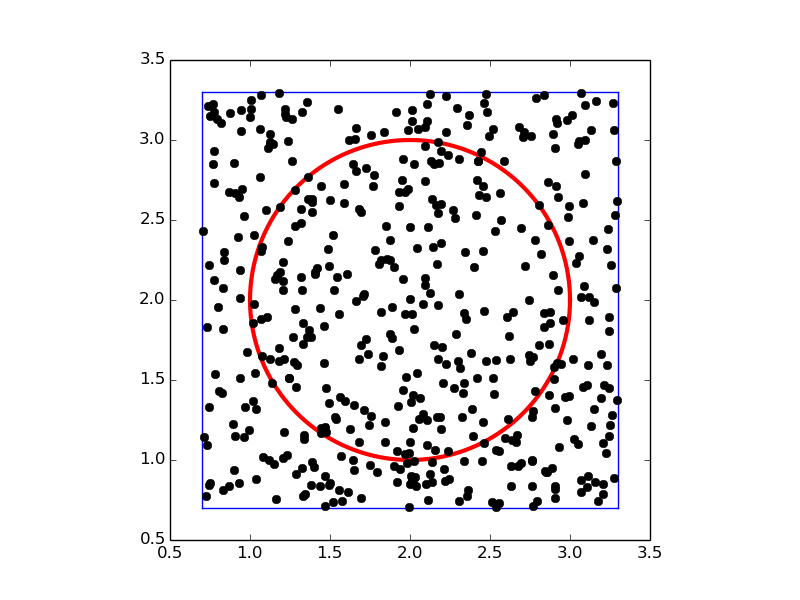
To get an idea of the method, consider a circular domain \(\Omega\) embedded in a rectangle as shown below. A collection of random points is illustrated by black dots.

Implementation

A Python function implementing \(\int_\Omega f(x,y)dxdy\) can be written like this:

import numpy as np

def MonteCarlo_double(f, g, x0, x1, y0, y1, n):
    """
    Monte Carlo integration of f over a domain g>=0, embedded
    in a rectangle [x0,x1]x[y0,y1]. n^2 is the number of
    random points.
    """
    # Draw n**2 random points in the rectangle
    x = np.random.uniform(x0, x1, n)
    y = np.random.uniform(y0, y1, n)
    # Compute sum of f values inside the integration domain
    f_mean = 0
    num_inside = 0   # number of x,y points inside domain (g>=0)
    for i in range(len(x)):
        for j in range(len(y)):
            if g(x[i], y[j]) >= 0:
                num_inside += 1
                f_mean += f(x[i], y[j])
    f_mean = f_mean/float(num_inside)
    area = num_inside/float(n**2)*(x1 - x0)*(y1 - y0)
    return area*f_mean

(See the file MC_double.py.)

Verification

A simple test case is to check the area of a rectangle \([0,2]\times[3,4.5]\) embedded in a rectangle \([0,3]\times [2,5]\). The right answer is 3, but Monte Carlo integration is, unfortunately, never exact so it is impossible to predict the output of the algorithm. All we know is that the estimated integral should approach 3 as the number of random points goes to infinity. Also, for a fixed number of points, we can run the algorithm several times and get different numbers that fluctuate around the exact value, since different sample points are used in different calls to the Monte Carlo integration algorithm.

The area of the rectangle can be computed by the integral \(\int_0^2\int_3^{4.5} dydx\), so in this case we identify \(f(x,y)=1\), and the \(g\) function can be specified as (e.g.) 1 if \((x,y)\) is inside \([0,2]\times[3,4.5]\) and \(-1\) otherwise. Here is an example on how we can utilize the MonteCarlo_double function to compute the area for different number of samples:

>>> from MC_double import MonteCarlo_double
>>> def g(x, y):
...     return (1 if (0 <= x <= 2 and 3 <= y <= 4.5) else -1)
...
>>> MonteCarlo_double(lambda x, y: 1, g, 0, 3, 2, 5, 100)
2.9484
>>> MonteCarlo_double(lambda x, y: 1, g, 0, 3, 2, 5, 1000)
2.947032
>>> MonteCarlo_double(lambda x, y: 1, g, 0, 3, 2, 5, 1000)
3.0234600000000005
>>> MonteCarlo_double(lambda x, y: 1, g, 0, 3, 2, 5, 2000)
2.9984580000000003
>>> MonteCarlo_double(lambda x, y: 1, g, 0, 3, 2, 5, 2000)
3.1903469999999996
>>> MonteCarlo_double(lambda x, y: 1, g, 0, 3, 2, 5, 5000)
2.986515

We see that the values fluctuate around 3, a fact that supports a correct implementation, but in principle, bugs could be hidden behind the inaccurate answers.

It is mathematically known that the standard deviation of the Monte Carlo estimate of an integral converges as \(n^{-1/2}\), where \(n\) is the number of samples. This kind of convergence rate estimate could be used to verify the implementation, but this topic is beyond the scope of this book.

Test function for function with random numbers

To make a test function, we need a unit test that has identical behavior each time we run the test. This seems difficult when random numbers are involved, because these numbers are different every time we run the algorithm, and each run hence produces a (slightly) different result. A standard way to test algorithms involving random numbers is to fix the seed of the random number generator. Then the sequence of numbers is the same every time we run the algorithm. Assuming that the MonteCarlo_double function works, we fix the seed, observe a certain result, and take this result as the correct result. Provided the test function always uses this seed, we should get exactly this result every time the MonteCarlo_double function is called. Our test function can then be written as shown below.

def test_MonteCarlo_double_rectangle_area():
    """Check the area of a rectangle."""
    def g(x, y):
        return (1 if (0 <= x <= 2 and 3 <= y <= 4.5) else -1)

    x0 = 0;  x1 = 3;  y0 = 2;  y1 = 5  # embedded rectangle
    n = 1000
    np.random.seed(8)      # must fix the seed!
    I_expected = 3.121092  # computed with this seed
    I_computed = MonteCarlo_double(
        lambda x, y: 1, g, x0, x1, y0, y1, n)
    assert abs(I_expected - I_computed) < 1E-14

(See the file MC_double.py.)

Integral over a circle

The test above involves a trivial function \(f(x,y)=1\). We should also test a non-constant \(f\) function and a more complicated domain. Let \(\Omega\) be a circle at the origin with radius 2, and let \(f=\sqrt{x^2 + y^2}\). This choice makes it possible to compute an exact result: in polar coordinates, \(\int_\Omega f(x,y)dxdy\) simplifies to \(2\pi\int_0^2 r^2dr = 16\pi/3\). We must be prepared for quite crude approximations that fluctuate around this exact result. As in the test case above, we experience better results with larger number of points. When we have such evidence for a working implementation, we can turn the test into a proper test function. Here is an example:

def test_MonteCarlo_double_circle_r():
    """Check the integral of r over a circle with radius 2."""
    def g(x, y):
        xc, yc = 0, 0  # center
        R = 2          # radius
        return  R**2 - ((x-xc)**2 + (y-yc)**2)

    # Exact: integral of r*r*dr over circle with radius R becomes
    # 2*pi*1/3*R**3
    import sympy
    r = sympy.symbols('r')
    I_exact = sympy.integrate(2*sympy.pi*r*r, (r, 0, 2))
    print 'Exact integral:', I_exact.evalf()
    x0 = -2;  x1 = 2;  y0 = -2;  y1 = 2
    n = 1000
    np.random.seed(6)
    I_expected = 16.7970837117376384  # Computed with this seed
    I_computed = MonteCarlo_double(
        lambda x, y: np.sqrt(x**2 + y**2),
        g, x0, x1, y0, y1, n)
    print 'MC approximation %d samples): %.16f' % (n**2, I_computed)
    assert abs(I_expected - I_computed) < 1E-15

(See the file MC_double.py.)

Exercises

Compute by hand the area composed of two trapezoids (of equal width) that approximates the integral \(\int_1^3 2x^3dx\). Make a test function that calls the trapezoidal function in trapezoidal.py and compares the return value with the hand-calculated value.

Solution. The code may be written as follows

from trapezoidal import trapezoidal

def test_trapezoidal():
    def f(x):
        return 2*x**3
    a = 1;  b = 3
    n = 2
    numerical = trapezoidal(f, a, b, n)
    hand = 44.0
    error = abs(numerical - hand)
    tol = 1E-14
    assert error < tol, error

test_trapezoidal()

Filename: trapezoidal_test_func.py.

Compute by hand the area composed of two rectangles (of equal width) that approximates the integral \(\int_1^3 2x^3dx\). Make a test function that calls the midpoint function in midpoint.py and compares the return value with the hand-calculated value.

Solution. The code may be written as follows

from midpoint import midpoint

def test_midpoint():
    def f(x):
        return 2*x**3
    a = 1;  b = 3;
    n = 2
    numerical = midpoint(f, a, b, n)
    hand = 38.0
    error = abs(numerical - hand)
    tol = 1E-14
    assert error < tol, error

test_midpoint()

Filename: midpoint_test_func.py.

Apply the trapezoidal and midpoint functions to compute the integral \(\int_2^6 x(x -1)dx\) with 2 and 100 subintervals. Compute the error too.

Solution. The code may be written as follows

from trapezoidal import trapezoidal
from midpoint import midpoint

def f(x):
    return x*(x-1)

a = 2;  b = 6;
n = 100

numerical_trap = trapezoidal(f, a, b, n)
numerical_mid  = midpoint(f, a, b, n)

# Compute exact integral by sympy
import sympy as sp
x = sp.symbols('x')
F = sp.integrate(f(x))
exact = F.subs(x, b) - F.subs(x, a)
exact = exact.evalf()

error_trap = abs(numerical_trap - exact)
error_mid  = abs(numerical_mid - exact)

print 'For n = %d, we get:' % (n)
print 'Numerical trapezoid: %g , Error: %g' % \
                                 (numerical_trap,error_trap)
print 'Numerical midpoint: %g , Error: %g' % \
                                 (numerical_mid,error_mid)

In the code, we have taken the opportunity to show how commenting often is used to switch between two code fragments, typically single statements. The alternatives n = 2 and n = 100 are switched by removing/adding the comment sign #, before running the code anew. Another alternative would of course be to ask the user for the value of n. Running the program with n = 2, produces the following printout:

For n = 2, we get:
Numerical trapezoid: 56 , Error: 2.667
Numerical midpoint: 52 , Error: 1.333

while running it with n = 100 gives:

For n = 100, we get:
Numerical trapezoid: 53.3344 , Error: 0.0014
Numerical midpoint: 53.3328 , Error: 0.0002

The analytical value of the integral is 53.333 (rounded).

Filename: integrate_parabola.py.

We consider integrating the sine function: \(\int_0^b \sin (x)dx\).

a) Let \(b=\pi\) and use two intervals in the trapezoidal and midpoint method. Compute the integral by hand and illustrate how the two numerical methods approximates the integral. Compare with the exact value.

Solution. Analytically, the integral computes to 2. By hand, with the trapezoidal method, we get 1.570. Graphically (Figure The integral computed with the trapezoidal method (n = 2)), it is clear that the numerical approach will have to under-estimate the true result.

The area under the blue graph in Figure The integral computed with the trapezoidal method (n = 2) corresponds to the “true” area under the graph of the integrand. The area under the red graph corresponds to what you get with the trapezoidal method and two intervals.

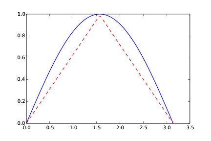
The integral computed with the trapezoidal method (n = 2)

By hand, with the midpoint method, we get 2.221. Graphically (Figure The integral computed with the midpoint method (n = 2)), we might see that the numerical approach will have to over-estimate the true result. Again, the area under the blue graph in Figure The integral computed with the midpoint method (n = 2) corresponds to the “true” area under the graph of the integrand. The area under the red graph corresponds to what you get with the midpoint method and two intervals.

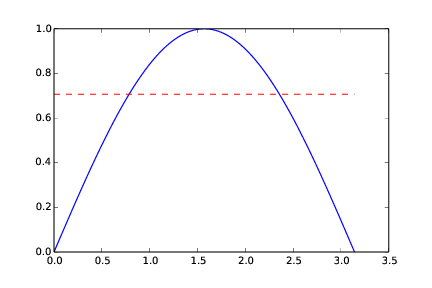
The integral computed with the midpoint method (n = 2)

b) Do a) when \(b=2\pi\).

Solution. Analytically, the integral computes to zero. In this case, both numerical methods will correctly calculate the integral to zero even with just two intervals! Graphically, we see that they arrive at zero for “different reasons”. The trapezoidal method constructs both its trapezoids by use of the function (integrand) value at the midpoint of the whole interval. However, there the integrand crosses the x-axis, i.e. it evaluates to zero. The “area” computed by the trapezoidal method becomes the zero area located “between” the green graph and the x-axis in Figure The integral computed with the trapezoidal and midpoint method (n = 2). The midpoint method computes the areas of two rectangles (red graph in Figure The integral computed with the trapezoidal and midpoint method (n = 2)), but since the signs of these equal areas differ, they add to zero.

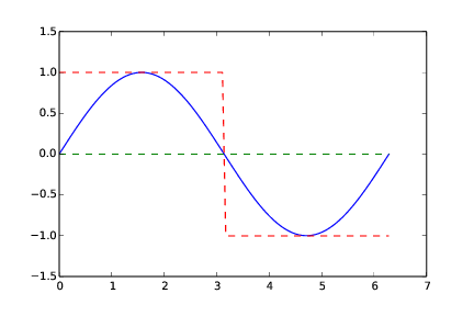
The integral computed with the trapezoidal and midpoint method (n = 2)

Filename: integrate_sine.pdf.

Modify the file test_trapezoidal.py such that the three tests are applied to the function midpoint implementing the midpoint method for integration.

Solution. Note that also the midpoint method will do an exact (to within machine precision) integration when the integrand is a straight line. This is so, since the errors from each rectangle will cancel. The code reads:

from midpoint import midpoint

def test_midpoint_one_exact_result():
    """Compare one hand-computed result."""
    from math import exp
    v = lambda t: 3*(t**2)*exp(t**3)
    n = 2
    numerical = midpoint(v, 0, 1, n)
    exact = 1.3817914596908085
    err = abs(exact - numerical)
    tol = 1E-14
    assert err < tol, err

def test_midpoint_linear():
    """Check that linear functions are integrated exactly"""
    # ...they should, since errros from each rectangle cancel
    f = lambda x: 6*x - 4
    F = lambda x: 3*x**2 - 4*x  # Anti-derivative
    a = 1.2;  b = 4.4
    exact = F(b) - F(a)
    tol = 1E-14
    for n in 2, 20, 21:
        numerical = midpoint(f, a, b, n)
        err = abs(exact - numerical)
        assert err < tol, 'n = %d, err = %g' % (n,err)

def test_midpoint_conv_rate():
    """Check empirical convergence rates against the expected -2."""
    from math import exp
    v = lambda t: 3*(t**2)*exp(t**3)
    V = lambda t: exp(t**3)
    a = 1.1;  b = 1.9
    r = convergence_rates(v, V, a, b, 14)
    print r
    tol = 0.01
    assert (abs(r[-1]) - 2) < tol, r[-4:]

def convergence_rates(f, F, a, b, num_experiments=14):
    from math import log
    from numpy import zeros
    exact = F(b) - F(a)
    n = zeros(num_experiments, dtype=int)
    E = zeros(num_experiments)
    r = zeros(num_experiments-1)
    for i in range(num_experiments):
        n[i] = 2**(i+1)
        numerical = midpoint(f, a, b, n[i])
        E[i] = abs(exact - numerical)
        if i > 0:
            r_im1 = log(E[i]/E[i-1])/log(float(n[i])/n[i-1])
            r[i-1] = float('%.2f' % r_im1)  # Truncate, two decimals
    return r

test_midpoint_one_exact_result()
test_midpoint_linear()
test_midpoint_conv_rate()

Filename: test_midpoint.py.

The trapezoidal method integrates linear functions exactly, and this property was used in the test function test_trapezoidal_linear in the file test_trapezoidal.py. Change the function used in the section sec:integrals:testprocs to \(f(x)=6\cdot 10^8 x - 4\cdot 10^6\) and rerun the test. What happens? How must you change the test to make it useful? How does the convergence rate test behave? Any need for adjustment?

Solution. With the new function given, we get the error message that includes:

AssertionError: n = 2, err = 9.53674e-07

The numerical calculation then obviously differs from the exact value by more than what is specified in the tolerance tol. We may understand this by considering the new function, i.e., \(f(x)=6\cdot 10^8 x - 4\cdot 10^6\). Any rounding error in \(x\) will get magnified big time by the factor \(6\cdot 10^8\) in front, i.e. the slope of the line. This makes the numerical calculation more inaccurate than previously. To fix this problem, we have several options. One possibility is to relax the tolerance, but this is not very satisfactory. After all, the calculation is supposed to be “exact” for a straight line. Another alternative is to introduce a new integration variable such that we scale the interval \([a,b]\) into \([\frac{a}{6\cdot 10^8},\frac{b}{6\cdot 10^8}]\), as this will neutralize the huge factor in front of \(x\), bringing the accuracy back to where it was previously. This alternative is implemented in test_trapezoidal2.py.

from trapezoidal import trapezoidal

def test_trapezoidal_linear_scale():
    """Check that linear functions are integrated exactly"""
    f = lambda x: 6E8*x - 4E6
    F = lambda x: 3E8*x**2 - 4E6*x  # Anti-derivative
    #a = 1.2;  b = 4.4
    a = 1.2/6E8;  b = 4.4/6E8       # Scale interval down
    exact = F(b) - F(a)
    tol = 1E-14
    for n in 2, 20, 21:
        numerical = trapezoidal(f, a, b, n)
        err = abs(exact - numerical)
        msg = 'n = %d, err = %g' % (n, err)
        assert err < tol, msg
        print msg

A third alternative is to use the module decimal that comes with Python, which allows number precision to be altered by the programmer. An alternative, better suited for numerical computing, is the mpmath module in SymPy (since it supports standard mathematical functions such as sin and cos with arbitrary precision, while decimal can only the standard arithmetics with arbitrary precision).

from trapezoidal import trapezoidal

def test_trapezoidal_linear_scale():
    """Check that linear functions are integrated exactly"""
    f = lambda x: 6E8*x - 4E6
    F = lambda x: 3E8*x**2 - 4E6*x  # Anti-derivative
    #a = 1.2;  b = 4.4
    a = 1.2/6E8;  b = 4.4/6E8       # Scale interval down
    exact = F(b) - F(a)
    tol = 1E-14
    for n in 2, 20, 21:
        numerical = trapezoidal(f, a, b, n)
        err = abs(exact - numerical)
        msg = 'n = %d, err = %g' % (n, err)
        assert err < tol, msg
        print msg

def test_trapezoidal_linear_reldiff():
    """
    Check that linear functions are integrated exactly.
    Use relative and not absolute difference.
    """
    f = lambda x: 6E8*x - 4E6
    F = lambda x: 3E8*x**2 - 4E6*x  # Anti-derivative
    a = 1.2;  b = 4.4               # Scale interval down
    exact = F(b) - F(a)
    tol = 1E-14
    for n in 2, 20, 21:
        numerical = trapezoidal(f, a, b, n)
        err = abs(exact - numerical)/exact
        msg = 'n = %d, err = %g' % (n, err)
        assert err < tol, msg
        print msg

def test_trapezoidal_conv_rate():
    """Check empirical convergence rates against the expected -2."""
    #from math import exp
    f = lambda x: 6E8*x - 4E6
    F = lambda x: 3E8*x**2 - 4E6*x  # Anti-derivative
    a = 1.1;  b = 1.9
    r = convergence_rates(f, F, a, b, 14)
    print r
    tol = 0.01
    assert abs(abs(r[-1]) - 2) < tol, r[-4:]

def convergence_rates(f, F, a, b, num_experiments=14):
    from math import log
    from numpy import zeros
    exact = F(b) - F(a)
    n = zeros(num_experiments, dtype=int)
    E = zeros(num_experiments)
    r = zeros(num_experiments-1)
    for i in range(num_experiments):
        n[i] = 2**(i+1)
        numerical = trapezoidal(f, a, b, n[i])
        E[i] = abs(exact - numerical)
        print E[i]
        if i > 0:
            r_im1 = log(E[i]/E[i-1])/log(float(n[i])/n[i-1])
            r[i-1] = float('%.2f' % r_im1)  # Truncate, two decimals
    return r

test_trapezoidal_linear_scale()
test_trapezoidal_linear_reldiff()
test_trapezoidal_conv_rate()

The best alternative, however, is to consider relative differences instead of absolute differences. That is, we compute (exact - numerical)/exact instead of just exact - numerical. This relative error is \(10^{-16}\) even if we compute with very big numbers.

def test_trapezoidal_linear_reldiff():
    """
    Check that linear functions are integrated exactly.
    Use relative and not absolute difference.
    """
    f = lambda x: 6E8*x - 4E6
    F = lambda x: 3E8*x**2 - 4E6*x  # Anti-derivative
    a = 1.2;  b = 4.4               # Scale interval down
    exact = F(b) - F(a)
    tol = 1E-14
    for n in 2, 20, 21:
        numerical = trapezoidal(f, a, b, n)
        err = abs(exact - numerical)/exact
        msg = 'n = %d, err = %g' % (n, err)
        assert err < tol, msg
        print msg

def test_trapezoidal_conv_rate():
    """Check empirical convergence rates against the expected -2."""
    #from math import exp
    f = lambda x: 6E8*x - 4E6
    F = lambda x: 3E8*x**2 - 4E6*x  # Anti-derivative
    a = 1.1;  b = 1.9
    r = convergence_rates(f, F, a, b, 14)
    print r
    tol = 0.01
    assert abs(abs(r[-1]) - 2) < tol, r[-4:]

def convergence_rates(f, F, a, b, num_experiments=14):
    from math import log
    from numpy import zeros
    exact = F(b) - F(a)
    n = zeros(num_experiments, dtype=int)
    E = zeros(num_experiments)
    r = zeros(num_experiments-1)
    for i in range(num_experiments):
        n[i] = 2**(i+1)
        numerical = trapezoidal(f, a, b, n[i])
        E[i] = abs(exact - numerical)
        print E[i]
        if i > 0:
            r_im1 = log(E[i]/E[i-1])/log(float(n[i])/n[i-1])
            r[i-1] = float('%.2f' % r_im1)  # Truncate, two decimals
    return r

Computing convergence rates is not meaningful in this test, because the error is mathematically zero.

Filename: test_trapezoidal2.py.

We want to test how the trapezoidal function works for the integral \(\int_0^4\sqrt{x}dx\). Two of the tests in test_trapezoidal.py are meaningful for this integral. Compute by hand the result of using 2 or 3 trapezoids and modify the test_trapezoidal_one_exact_result function accordingly. Then modify test_trapezoidal_conv_rate to handle the square root integral.

Solution. Adjustments to the code are made according to the remark below and hand calculations are written into the code. The code then reads:

from trapezoidal import trapezoidal

def test_trapezoidal_one_exact_result():
    """Compare one hand-computed result."""
    f = lambda x: x**0.5
    tol = 1E-14
    exact = [4.82842712474619, 5.050258266979605] # n=2, n=3
    for n in [2, 3]:
        numerical = trapezoidal(f, 0, 4, n)
        err = abs(exact[n-2] - numerical)
        assert err < tol, err

def test_trapezoidal_conv_rate():
    """Check empirical convergence rates against the expected -2."""
    from math import exp
    f = lambda x: x**0.5
    F = lambda x: (2.0/3)*x**(3.0/2)
    a = 0.0 + 0.1;  b = 4.0         # a adjusted by 0.1
    r = convergence_rates(f, F, a, b, 14)
    print r
    tol = 0.01
    assert abs(abs(r[-1]) - 2) < tol, r[-4:]

def convergence_rates(f, F, a, b, num_experiments=14):
    from math import log
    from numpy import zeros
    exact = F(b) - F(a)
    n = zeros(num_experiments, dtype=int)
    E = zeros(num_experiments)
    r = zeros(num_experiments-1)
    for i in range(num_experiments):
        n[i] = 2**(i+1)
        numerical = trapezoidal(f, a, b, n[i])
        E[i] = abs(exact - numerical)
        if i > 0:
            r_im1 = log(E[i]/E[i-1])/log(float(n[i])/n[i-1])
            r[i-1] = float('%.2f' % r_im1)  # Truncate to two decimals
    return r

test_trapezoidal_one_exact_result()
test_trapezoidal_conv_rate()

Filename: test_trapezoidal3.py.

Remarks

The convergence rate test fails. Printing out r shows that the actual convergence rate for this integral is \(-1.5\) and not \(-2\). The reason is that the error in the trapezoidal method is \(-(b-a)^3n^{-2}f''(\xi)\) for some (unknown) \(\xi\in [a,b]\). With \(f(x)=\sqrt{x}\), \(f''(\xi)\rightarrow -\infty\) as \(\xi\rightarrow 0\), pointing to a potential problem in the size of the error. Running a test with \(a>0\), say \(\int_{0.1}^4\sqrt{x}dx\) shows that the convergence rate is indeed restored to -2.

Exercise 37: Rectangle methods

The midpoint method divides the interval of integration into equal-sized subintervals and approximates the integral in each subinterval by a rectangle whose height equals the function value at the midpoint of the subinterval. Instead, one might use either the left or right end of the subinterval as illustrated in Figure Illustration of the rectangle method with evaluating the rectangle height by either the left or right point. This defines a rectangle method of integration. The height of the rectangle can be based on the left or right end or the midpoint.

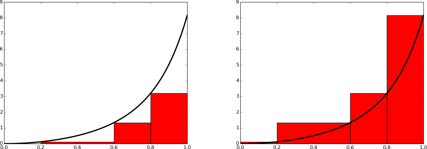
Illustration of the rectangle method with evaluating the rectangle height by either the left or right point

a) Write a function rectangle(f, a, b, n, height='left') for computing an integral \(\int_a^bf(x)dx\) by the rectangle method with height computed based on the value of height, which is either

left, right, or mid.

Solution. Placing the code for both a and b into one file, the code may read:

def rectangle(f, a, b, n, height='left'):
    """Uses a rectangle method for integrating f. The height of
    each rectangle is computed either at the left end, middle or
    right end of each sub-interval"""
    h = float(b-a)/n
    if height == 'left':
        start = a
    elif height == 'mid':
        start = a + h/2.0
    else:      # Must be right end
        start = a + h
    result = 0
    for i in range(n):
        result += f((start) + i*h)
    result *= h
    return result

def test_rectangle_one_exact_result():
    """Compare one hand-computed result."""
    from math import exp
    v = lambda t: 3*(t**2)*exp(t**3)
    method = ['left', 'mid', 'right']
    n = 2
    exact = [0.4249306699000599, 1.3817914596908085, \
                                           4.5023534125886275]
    tol = 1E-14
    for i in range(len(method)):
        numerical = rectangle(v, 0, 1, n, method[i])
        err = abs(exact[i] - numerical)
        assert err < tol, err

def test_rectangle_linear():
    """Check that linear functions are integrated exactly
    (with midpoint) or with a known correctable error (left
    and right)"""
    method = ['left', 'mid', 'right']
    f = lambda x: 6*x - 4
    slope = 6
    F = lambda x: 3*x**2 - 4*x  # Anti-derivative
    # From the slope of f (i.e. 6), we know that left will
    # under-estimate the inegral by C (given below), while
    # right will over-estimate by C
    a = 1.2;  b = 4.4
    exact = F(b) - F(a)
    #tol = 1E-14
    tol = 1E-13        # Slightly relaxed compared to previously
    for n in 2, 20, 21:
        h = float(b-a)/n
        C = n*(0.5*slope*h**2)    # Correction term for left/right
        for i in range(len(method)):
            numerical = rectangle(f, a, b, n, method[i])
            if (method[i] == 'left'):
                numerical += C
            elif (method[i] == 'right'):
                numerical -= C
            err = abs(exact - numerical)
            assert err < tol, 'n = %d, err = %g' % (n,err)

def test_rectangle_conv_rate():
    """Check empirical convergence rates against the expected rate,
    which is -2 for midpoint and -1 for left and right."""
    from math import exp
    method = ['left', 'mid', 'right']
    v = lambda t: 3*(t**2)*exp(t**3)
    V = lambda t: exp(t**3)
    a = 1.1;  b = 1.9
    tol = 0.01
    for i in range(len(method)):
        r = convergence_rates(v, V, a, b, method[i], 14)
        print r
        if (method[i] == 'left') or (method[i] == 'right'):
            assert abs(abs(r[-1]) - 1) < tol, r[-4:]
        else:
            assert abs(abs(r[-1]) - 2) < tol, r[-4:]

def convergence_rates(f, F, a, b, height, num_experiments=14):
    from math import log
    from numpy import zeros
    exact = F(b) - F(a)
    n = zeros(num_experiments, dtype=int)
    E = zeros(num_experiments)
    r = zeros(num_experiments-1)
    for i in range(num_experiments):
        n[i] = 2**(i+1)
        numerical = rectangle(f, a, b, n[i], height)
        E[i] = abs(exact - numerical)
        if i > 0:
            r_im1 = log(E[i]/E[i-1])/log(float(n[i])/n[i-1])
            r[i-1] = float('%.2f' % r_im1)  # Truncate to two decimals
    return r

test_rectangle_one_exact_result()
test_rectangle_linear()
test_rectangle_conv_rate()

b) Write three test functions for the three unit test procedures described in the section sec:integrals:testprocs. Make sure you test for height equal to left, right, and mid. You may call the midpoint function for checking the result when height=mid.

Hint. Edit test_trapezoidal.py.

Solution. See code above.

Filename: rectangle_methods.py.

Exercise 38: Adaptive integration

Suppose we want to use the trapezoidal or midpoint method to compute an integral \(\int_a^b f(x)dx\) with an error less than a prescribed tolerance \(\epsilon\). What is the appropriate size of \(n\)?

To answer this question, we may enter an iterative procedure where we compare the results produced by \(n\) and \(2n\) intervals, and if the difference is smaller than \(\epsilon\), the value corresponding to \(2n\) is returned. Otherwise, we halve \(n\) and repeat the procedure.

Hint. It may be a good idea to organize your code so that the function adaptive_integration can be used easily in future programs you write.

a) Write a function

adaptive_integration(f, a, b, eps, method=midpoint)

that implements the idea above (eps corresponds to the tolerance \(\epsilon\), and method can be midpoint or trapezoidal).

Solution. Easing the answers to the whole of this exercise, as well as preparing for easy use of adaptive integration in future programs, we organize the coding of tasks a, b and c into one file, making it a module. The code then reads:

from numpy import linspace, zeros, sqrt, log
from trapezoidal import trapezoidal
from midpoint import midpoint

def adaptive_integration(f, a, b, eps, method='midpoint'):
    n_limit = 1000000   # Just a choice (used to avoid inf loop)
    n = 2
    if method == 'trapezoidal':
        integral_n  = trapezoidal(f, a, b, n)
        integral_2n = trapezoidal(f, a, b, 2*n)
        diff = abs(integral_2n - integral_n)
        print 'trapezoidal diff: ', diff
        while (diff > eps) and (n < n_limit):
            integral_n  = trapezoidal(f, a, b, n)
            integral_2n = trapezoidal(f, a, b, 2*n)
            diff = abs(integral_2n - integral_n)
            print 'trapezoidal diff: ', diff
            n *= 2
    elif method == 'midpoint':
        integral_n  = midpoint(f, a, b, n)
        integral_2n = midpoint(f, a, b, 2*n)
        diff = abs(integral_2n - integral_n)
        print 'midpoint diff: ', diff
        while (diff > eps) and (n < n_limit):
            integral_n  = midpoint(f, a, b, n)
            integral_2n = midpoint(f, a, b, 2*n)
            diff = abs(integral_2n - integral_n)
            print 'midpoint diff: ', diff
            n *= 2
    else:
        print 'Error - adaptive integration called with unknown par'
    # Now we check if acceptable n was found or not
    if diff <= eps:   # Success
        print 'The integral computes to: ', integral_2n
        return n
    else:
        return -n   # Return negative n to tell "not found"

def application():
    """...Tasks b) and c)"""

    def f(x):
        return x**2
    def g(x):
        return sqrt(x)

    #eps = 1E-1           # Just switch between these two eps values
    eps = 1E-10
    #a = 0.0
    a = 0.0 + 0.01;       # If we adjust a, sqrt(x) is handled easily
    b = 2.0
    # ...f
    n = adaptive_integration(f, a, b, eps, 'midpoint')
    if n > 0:
        print 'Sufficient n is: %d' % (n)
    else:
        print 'No n was found in %d iterations' % (n_limit)

    n = adaptive_integration(f, a, b, eps, 'trapezoidal')
    if n > 0:
        print 'Sufficient n is: %d' % (n)
    else:
        print 'No n was found in %d iterations' % (n_limit)

    # ...g
    n = adaptive_integration(g, a, b, eps, 'midpoint')
    if n > 0:
        print 'Sufficient n is: %d' % (n)
    else:
        print 'No n was found in %d iterations' % (n_limit)

    n = adaptive_integration(g, a, b, eps, 'trapezoidal')
    if n > 0:
        print 'Sufficient n is: %d' % (n)
    else:
        print 'No n was found in %d iterations' % (n_limit)

    # Task c, make plot for both midpoint and trapezoidal
    eps = linspace(1E-1,10E-10,10)
    n_m = zeros(len(eps))
    n_t = zeros(len(eps))
    for i in range(len(n_m)):
        n_m[i] = adaptive_integration(g, a, b, eps[i], 'midpoint')
        n_t[i] = adaptive_integration(g, a, b, eps[i], 'trapezoidal')

    import matplotlib.pyplot as plt
    plt.plot(log(eps),n_m,'b-',log(eps),n_t,'r-')
    plt.xlabel('log(eps)')
    plt.ylabel('n for midpoint (blue) and trapezoidal (red)')
    plt.show()
    print n
    print eps

if __name__ == '__main__':
    application()

b) Test the method on \(\int_0^2x^2dx\) and \(\int_0^2\sqrt{x}dx\) for \(\epsilon = 10^{-1}, 10^{-10}\) and write out the exact error.

Solution. See the code above. Note that, in our suggested code, it is foreseen that the programmer switches between the two epsilon values by use of commenting, i.e. adding/removing #. This may of course be avoided, if desirable, by asking the user for epsilon.

c) Make a plot of \(n\) versus \(\epsilon \in [10^{-1}, 10^{-10}]\) for \(\int_0^2\sqrt{x}dx\). Use logarithmic scale for \(\epsilon\).

Solution. From Figure Showing n as a function of log(eps) when is computed by the midpoint (blue) and the trapezoidal (red) method, we see that the stricter the value of epsilon, the larger the difference between the midpoint and the trapezoidal methods. For a given value for epsilon, the midpoint method comes within the tolerance with fewer intervals (lower value of n) than does the trapezoidal method. This should be expected, since the midpoint method is somewhat more accurate than the trapezoidal method.

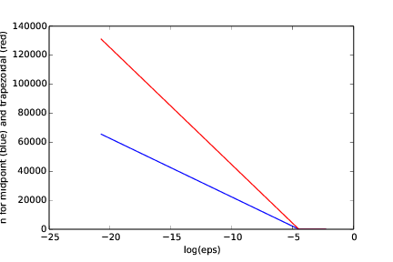
Showing n as a function of log(eps) when \(\int_0^2\sqrt{x}dx\) is computed by the midpoint (blue) and the trapezoidal (red) method

One way of producing this plot, is by using the code lines included at the end of adaptive_integration.py (see the above).

Filename: adaptive_integration.py.

Remarks

The type of method explored in this exercise is called adaptive, because it tries to adapt the value of \(n\) to meet a given error criterion. The true error can very seldom be computed (since we do not know the exact answer to the computational problem), so one has to find other indicators of the error, such as the one here where the changes in the integral value, as the number of intervals is doubled, is taken to reflect the error.

Exercise 39: Integrating x raised to x

Consider the integral

\[I = \int_0^4 x^x\,dx\thinspace .\]

The integrand \(x^x\) does not have an anti-derivative that can be expressed in terms of standard functions (visit http://wolframalpha.com and type integral(x**x,x) to convince yourself that our claim is right. Note that Wolfram alpha does give you an answer, but that answer is an approximation, it is not exact. This is because Wolfram alpha too uses numerical methods to arrive at the answer, just as you will in this exercise). Therefore, we are forced to compute the integral by numerical methods. Compute a result that is right to four digits.

Hint. Use ideas from Exercise 38: Adaptive integration.

Solution. When the function adaptive_integration is available, the code may be written as:

from adaptive_integration import adaptive_integration

def f(x):
    return x**x

eps = 1E-4
a = 0.0;  b = 2.0

# Choose midpoint method
n = adaptive_integration(f, a, b, eps, 'midpoint')
if n > 0:
    print 'Sufficient n is: %d' % (n)
else:
    # The negative n is returned to signal that the upper limit of n
    # was passed
    print 'No n was found in %d iterations' % (abs(n))

Remember that adaptive_integration prints out the computed integral, so no effort in that respect is required here.

Running the program, gives a printout to the screen showing how diff gets smaller and smaller each time. The final two lines of the printout read:

The integral computes to: 2.83384395958
Sufficient n is: 256

The computed value may be compared to what Wolfram alpha gives. Remember that since we have not computed the exact error, we can not guarantee that the “result is right to four digits”. However, we have reason to believe that we “are close”. Typically, when it is known that the error measure used is not precise, the tolerance is made stricter.

Filename: integrate_x2x.py.

Exercise 40: Integrate products of sine functions

In this exercise we shall integrate

\[I_{j,k} = \int_{-\pi}^{\pi} \sin(jx)\sin(kx)dx,\]

where \(j\) and \(k\) are integers.

a) Plot \(\sin(x)\sin(2x)\) and \(\sin(2x)\sin(3x)\) for \(x\in ]-\pi,\pi]\) in separate plots. Explain why you expect \(\int_{-\pi}^{\pi}\sin x\sin 2x\,dx=0\) and \(\int_{-\pi}^{\pi}\sin 2x\sin 3x\,dx=0\).

b) Use the trapezoidal rule to compute \(I_{j,k}\) for \(j=1,\ldots,10\) and \(k=1,\ldots,10\).

Filename: products_sines.py.

Exercise 41: Revisit fit of sines to a function

This is a continuation of Exercise 28: Fit sines to straight line. The task is to approximate a given function \(f(t)\) on \([-\pi,\pi]\) by a sum of sines,

\[\tag{28} S_N(t) = \sum_{n=1}^{N} b_n \sin(nt)\thinspace .\]

We are now interested in computing the unknown coefficients \(b_n\) such that \(S_N(t)\) is in some sense the best approximation to \(f(t)\). One common way of doing this is to first set up a general expression for the approximation error, measured by “summing up” the squared deviation of \(S_N\) from \(f\):

\[E = \int_{-\pi}^{\pi}(S_N(t)-f(t))^2dt\thinspace .\]

We may view \(E\) as a function of \(b_1,\ldots,b_N\). Minimizing \(E\) with respect to \(b_1,\ldots,b_N\) will give us a best approximation, in the sense that we adjust \(b_1,\ldots,b_N\) such that \(S_N\) deviates as little as possible from \(f\).

Minimization of a function of \(N\) variables, \(E(b_1,\ldots,b_N)\) is mathematically performed by requiring all the partial derivatives to be zero:

\[\begin{split}\frac{\partial E}{\partial b_1} & = 0,\\ \frac{\partial E}{\partial b_2} & = 0,\\ &\vdots\\ \frac{\partial E}{\partial b_N} & = 0\thinspace .\end{split}\]

a) Compute the partial derivative \(\partial E/\partial b_1\) and generalize to the arbitrary case \(\partial E/\partial b_n\), \(1\leq n\leq N\).

Solution.

\[\frac{\partial E}{\partial b_1} = \frac{\partial}{\partial b_1} (\int_{-\pi}^{\pi}(S_N(t)-f(t))^2dt), \nonumber\]

\[= \int_{-\pi}^{\pi} \frac{\partial}{\partial b_1}((S_N(t)-f(t))^2dt), \nonumber\]

\[= 2\int_{-\pi}^{\pi} (S_N(t)-f(t))\sin(t)dt, \nonumber\]

where it has been assumed that the integrand is such that the partial derivative can be moved inside the integration.

We see that the partial derivative of \(E\) with respect to any one of the \(b\) coefficients will take on the same form, meaning that

\[\frac{\partial E}{\partial b_n} = 2\int_{-\pi}^{\pi} (S_N(t)-f(t))\sin(nt)dt, \nonumber\]

where \(1\leq n\leq N\).

b) Show that

\[b_n = \frac{1}{\pi}\int_{-\pi}^{\pi}f(t)\sin(nt)\,dt\thinspace .\]

Solution. Requiring

\[\frac{\partial E}{\partial b_n} = 0, \nonumber\]

means that the following must apply,

\[2\int_{-\pi}^{\pi} (S_N(t)-f(t))\sin(nt)dt = 0. \nonumber\]

This may be rewritten as

\[\int_{-\pi}^{\pi} S_N(t)\sin(nt)dt = \int_{-\pi}^{\pi} f(t)\sin(nt)dt \nonumber\]

or, if we insert the expression for \(S_N\), we get

\[\int_{-\pi}^{\pi} (\sum_{i=1}^{N} b_i \sin(it))\sin(nt)dt = \int_{-\pi}^{\pi} f(t)\sin(nt)dt, \nonumber\]

where the summation variable in \(S_N\) has been changed from \(n\) to \(i\), avoiding conflict with the \(n\) already present in \(\sin(nt)\).

Now, since

\[\int_{-\pi}^{\pi} \sin^2(nt)dt = \pi, \nonumber\]

while

\[\int_{-\pi}^{\pi} \sin(it)\sin(nt)dt = 0, \nonumber\]

when \(i \neq n\), we arrive at

\[b_n = \frac{1}{\pi}\int_{-\pi}^{\pi}f(t)\sin(nt)\,dt\thinspace .\]

c) Write a function integrate_coeffs(f, N, M) that computes \(b_1,\ldots,b_N\) by numerical integration, using \(M\) intervals in the trapezoidal rule.

Solution. Answers to all (programming) questions in this exercise are collected in one script which reads:

from numpy import linspace, zeros, pi, sin, exp
from trapezoidal import trapezoidal

def integrate_coeffs(f, N, M):
    b = zeros(N)
    left_end = -pi; right_end = pi
    for n in range(1, N+1):
        f_sin = lambda t: f(t)*sin(n*t)
        b[n-1] = (1/pi)*trapezoidal(f_sin, left_end, right_end, M)
    return b

def test_integrate_coeffs():
    """Check that sin(nt) are integrated exactly by trapezoidal"""
    def f(t):
        return 1
    tol = 1E-14
    N = 10
    M = 100
    b = integrate_coeffs(f, N, M)
    print b
    for i in range(0, 10):
        err = abs(b[i])  # Supposed to be zero
        assert err < tol, 'n = %d, err = %g' % (n,err)

def plot_approx(f, N, M, filename):
    def S_N(b,t):
        sum = 0
        for i in range(len(b)):
            sum += b[i]*sin((i+1)*t)
        return sum
    left_end = -pi;  right_end = pi
    time = linspace(-pi, pi, 100)
    y = f(time)
    b = integrate_coeffs(f, N, M)
    y_approx = S_N(b, time)

    import matplotlib.pyplot as plt
    plt.figure(); plt.plot(time, y, 'k-', time, y_approx, 'k--')
    plt.xlabel('t');  plt.ylabel('f (solid) and S (dashed)')
    plt.savefig(filename)

def application():
    def f(t):
        return (1/pi)*t
    N = 3
    M = 100
    b = integrate_coeffs(f, N, M)
    print b
    for N in [3, 6, 12, 24]:
        plot_filename = 'C:/Users/Svein/Desktop/S_whenNis' \
                                              + str(N) + '.pdf'
        plot_approx(f, N, M, plot_filename)
    def g(t):
        return exp(-(t-pi))
    plot_filename = 'C:/Users/Svein/Desktop/new_f_S_whenNis' \
                                              + str(100) + '.pdf'
    plot_approx(g, 100, M, plot_filename)

if __name__ == '__main__':
    application()
    test_integrate_coeffs()

d) A remarkable property of the trapezoidal rule is that it is exact for integrals \(\int_{-\pi}^{\pi}\sin nt\,dt\) (when subintervals are of equal size). Use this property to create a function test_integrate_coeff to verify the implementation of integrate_coeffs.

Solution. See code given above.

e) Implement the choice \(f(t) = \frac{1}{\pi}t\) as a Python function f(t) and call integrate_coeffs(f, 3, 100) to see what the optimal choice of \(b_1, b_2, b_3\) is.

Solution. See code given above. Running the script produces a printout of the following values for the \(b\) coefficients:

 0.63641032
-0.3178909
 0.2115779

f) Make a function plot_approx(f, N, M, filename) where you plot f(t) together with the best approximation \(S_N\) as computed above, using \(M\) intervals for numerical integration. Save the plot to a file with name filename.

Solution. See code given above.

g) Run plot_approx(f, N, M, filename) for \(f(t) = \frac{1}{\pi}t\) for \(N=3,6,12,24\). Observe how the approximation improves.

Solution. See code given above. Running the program will produce one plot (Figure The function and its approximation when , Figure The function and its approximation when , Figure The function and its approximation when and Figure The function and its approximation when ) for each value of \(N\). We see from the plots that the larger the \(N\), the better the approximation.

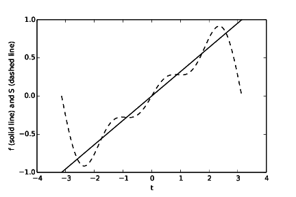
The function \(f(t)\) and its approximation \(S_N(t)\) when \(N = 3\)

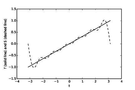
The function \(f(t)\) and its approximation \(S_N(t)\) when \(N = 6\)

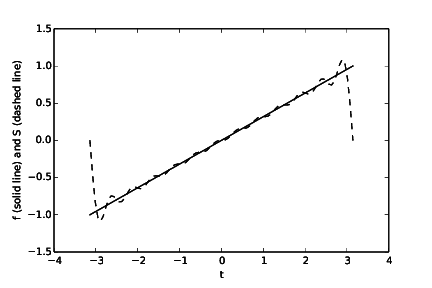
The function \(f(t)\) and its approximation \(S_N(t)\) when \(N = 12\)

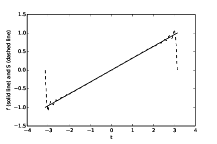
The function \(f(t)\) and its approximation \(S_N(t)\) when \(N = 24\)

h) Run plot_approx for \(f(t) = e^{-(t-\pi)}\) and \(N=100\). Observe a fundamental problem: regardless of \(N\), \(S_N(-\pi)=0\), not \(e^{2\pi}\approx 535\). (There are ways to fix this issue.)

Solution. See code given above. Running the program (also) produces the plot seen in Figure The new function and its approximation when . Clearly, the approximation is no good at the endpoints of the interval.

The new function \(f(t)\) and its approximation \(S_N(t)\) when \(N = 100\)

Filename: autofit_sines.py.

Exercise 42: Derive the trapezoidal rule for a double integral

Use ideas in the section sec:int:double:midpoint to derive a formula for computing a double integral \(\int_a^b\int_c^d f(x,y)dydx\) by the trapezoidal rule. Implement and test this rule.

Solution. We introduce a help function \(g(x)\) and write

\[\int_a^b \int_c^d f(x,y) dydx = \int_a^b g(x)dx,\quad g(x) = \int_c^d f(x,y) dy\thinspace .\]

Next, we apply the trapezoidal rule (The composite trapezoidal rule) to each of the integrals

\[\int_a^b g(x)dx,\quad g(x) = \int_c^d f(x,y) dy\thinspace .\]

Starting with \(g(x)=\int_c^d f(x,y)dy\), we introduce \(n_y\) intervals on \([c,d]\) with length \(h_y\). The trapezoidal rule for this integral then becomes

\[g(x) = \int_c^d f(x,y) dy \approx h_y \left[\frac{1}{2}f(x,c) + \sum_{j=1}^{n_y-1}f(x,y_j) + \frac{1}{2}f(x,d) \right],\]

with \(y_j = c + jh_y\). For the outer integral \(\int_a^b g(x)dx\), we get:

\[\int_a^b g(x)dx \approx h_x \left[\frac{1}{2}g(a) + \sum_{i=1}^{n_x-1}g(x_i) + \frac{1}{2}g(b) \right], \quad x_i=a + ih_x\thinspace .\]

Combining the formulas, we get the composite trapezoidal method for a double integral:

\[\int_a^b \int_c^d f(x,y) dydx \approx h_x \biggl[\frac{1}{2}\left(h_y \left[\frac{1}{2}f(a,c) + \sum_{j=1}^{n_y-1}f(a,y_j) + \frac{1}{2}f(a,d) \right]\right) + \nonumber\]

\[\quad \sum_{i=1}^{n_x-1}\left(h_y \left[\frac{1}{2}f(x_i,c) + \sum_{j=1}^{n_y-1}f(x_i,y_j) + \frac{1}{2}f(x_i,d) \right]\right)+\nonumber\]

\[\quad \frac{1}{2}\left(h_y \left[\frac{1}{2}f(b,c) + \sum_{j=1}^{n_y-1}f(b,y_j) + \frac{1}{2}f(b,d) \right]\right) \biggr]\nonumber\]

\[= h_xh_y \biggl[\frac{1}{4}\left(f(a,c) + f(a,d) + f(b,c) + f(b,d) \right) +\nonumber\]

\[\quad \frac{1}{2}\sum_{i=1}^{n_x-1}\left(f(a + ih_x,c) + f(a + ih_x,d)\right) + \nonumber\]

\[\quad \frac{1}{2}\sum_{j=1}^{n_y-1}\left(f(a,c + jh_y) + f(b,c + jh_y)\right) + \nonumber\]

\[\quad \sum_{i=1}^{n_x-1} \sum_{j=1}^{n_y-1} f(a + ih_x, c + jh_y)\biggr]\thinspace . \nonumber\]

The formula may be implemented and tested as shown in trapezoidal_double.py:

def trapezoidal_double(f, a, b, c, d, nx, ny):
    hx = (b - a)/float(nx)
    hy = (d - c)/float(ny)
    I = 0.25*(f(a, c) + f(a, d) + f(b, c) + f(b, d))
    Ix = 0
    for i in range(1, nx):
        xi = a + i*hx
        Ix += f(xi, c) + f(xi, d)
    I += 0.5*Ix
    Iy = 0
    for j in range(1, ny):
        yj = c + j*hy
        Iy += f(a, yj) + f(b, yj)
    I += 0.5*Iy
    Ixy = 0
    for i in range(1, nx):
        for j in range(1, ny):
            xi = a + i*hx
            yj = c + j*hy
            Ixy += f(xi, yj)
    I += Ixy
    I *= hx*hy
    return I

def test_trapezoidal_double():
    """Test that a linear function is integrated exactly."""
    def f(x, y):
        return 2*x + y

    a = 0;  b = 2;  c = 2;  d = 3
    import sympy
    x, y = sympy.symbols('x  y')
    I_expected = sympy.integrate(f(x, y), (x, a, b), (y, c, d))
    # Test three cases: nx < ny, nx = ny, nx > ny
    for nx, ny in (3, 5), (4, 4), (5, 3):
        I_computed = trapezoidal_double(f, a, b, c, d, nx, ny)
        tol = 1E-14
        #print I_expected, I_computed
        assert abs(I_computed - I_expected) < tol

if __name__ == '__main__':
    test_trapezoidal_double()

Filename: trapezoidal_double.py.

Exercise 43: Compute the area of a triangle by Monte Carlo integration

Use the Monte Carlo method from the section Monte Carlo integration for complex-shaped domains to compute the area of a triangle with vertices at \((-1,0)\), \((1,0)\), and \((3,0)\).

Solution. The program MC_triangle.py may be written as:

from MC_double import MonteCarlo_double

def g(x, y):
    """Utilize that triangle is symmetric about y-axis """
    return (1 if (0 <= y <= -3*abs(x) + 3) else -1 )

print MonteCarlo_double(lambda x, y: 1, g, -1, 1, 0, 3, 1000)

Filename: MC_triangle.py.