The first few steps
What is a program? And what is programming?
Today, most people are experienced with computer programs, typically programs such as Word, Excel, PowerPoint, Internet Explorer, and Photoshop. The interaction with such programs is usually quite simple and intuitive: you click on buttons, pull down menus and select operations, drag visual elements into locations, and so forth. The possible operations you can do in these programs can be combined in seemingly an infinite number of ways, only limited by your creativity and imagination.
Nevertheless, programs often make us frustrated when they cannot do what we wish. One typical situation might be the following. Say you have some measurements from a device, and the data are stored in a file with a specific format. You may want to analyze these data in Excel and make some graphics out of it. However, assume there is no menu in Excel that allows you to import data in this specific format. Excel can work with many different data formats, but not this one. You start searching for alternatives to Excel that can do the same and read this type of data files. Maybe you cannot find any ready-made program directly applicable. You have reached the point where knowing how to write programs on your own would be of great help to you! With some programming skills, you may write your own little program which can translate one data format to another. With that little piece of tailored code, your data may be read and analyzed, perhaps in Excel, or perhaps by a new program tailored to the computations that the measurement data demand.
The real power of computers can only be utilized if you can program them. By programming you can get the computer to do (most often!) exactly what you want. Programming consists of writing a set of instructions in a very specialized language that has adopted words and expressions from English. Such languages are known as programming or computer languages. The set of instructions is given to a program which can translate the meaning of the instructions into real actions inside the computer.
The purpose of this book is to teach you to write such instructions dedicated to solve mathematical and engineering problems by fundamental numerical methods.
There are numerous computer languages for different purposes. Within the engineering area, the most widely used computer languages are Python, MATLAB, Octave, Fortran, C, C++, and to some extent Maple, and Mathematica. How you write the instructions (i.e. the syntax) differs between the languages. Let us use an analogy.
Assume you are an international kind of person, having friends abroad in England, Russia and China. They want to try your favorite cake. What can you do? Well, you may write down the recipe in those three languages and send them over. Now, if you have been able to think correctly when writing down the recipe, and you have written the explanations according to the rules in each language, each of your friends will produce the same cake. Your recipe is the “computer program”, while English, Russian and Chinese represent the “computer languages” with their own rules of how to write things. The end product, though, is still the same cake. Note that you may unintentionally introduce errors in your “recipe”. Depending on the error, this may cause “baking execution” to stop, or perhaps produce the wrong cake. In your computer program, the errors you introduce are called bugs (yes, small insects! ...for historical reasons), and the process of fixing them is called debugging. When you try to run your program that contains errors, you usually get warnings or error messages. However, the response you get depends on the error and the programming language. You may even get no response, but simply the wrong “cake”. Note that the rules of a programming language have to be followed very strictly. This differs from languages like English etc., where the meaning might be understood even with spelling errors and “slang” included.
This book comes in two versions, one that is based on Python, and one based on Matlab. Both Python and Matlab represent excellent programming environments for scientific and engineering tasks. The version you are reading now, is the Python version.
Some of Python’s strong properties deserve mention here: Many global functions can be placed in only one file, functions are straightforwardly transferred as arguments to other functions, there is good support for interfacing C, C++ and Fortran code (i.e., a Python program may use code written in other languages), and functions explicitly written for scalar input often work fine (without modification) also with vector input. Another important thing, is that Python is available for free. It can be downloaded from the Internet and will run on most platforms.
Readers who want to expand their scientific programming skills beyond the introductory level of the present exposition, are encouraged to study the book A Primer on Scientific Programming with Python [Ref18]. This comprehensive book is as suitable for beginners as for professional programmers, and teaches the art of programming through a huge collection of dedicated examples. This book is considered the primary reference, and a natural extension, of the programming matters in the present book.
Some computer science terms
Note that, quite often, the terms script and scripting are used as synonyms for program and programming, respectively.
The inventor of the Perl programming language, Larry Wall, tried to explain the difference between script and program in a humorous way (from perl.com): Suppose you went back to `Ada Lovelace <http://en.wikipedia.org/wiki/Ada_Lovelace>`__ and asked her the difference between a script and a program. She’d probably look at you funny, then say something like: Well, a script is what you give the actors, but a program is what you give the audience. That Ada was one sharp lady... Since her time, we seem to have gotten a bit more confused about what we mean when we say scripting. It confuses even me, and I’m supposed to be one of the experts.
There are many other widely used computer science terms to pick up. Writing a program (or script or code) is often expressed as implementing the program. Executing a program means running the program. An algorithm is a recipe for how to construct a program. A bug is an error in a program, and the art of tracking down and removing bugs is called debugging.
Simulating or simulation refers to using a program to mimic processes in the real world, often through solving differential equations that govern the physics of the processes.
A Python program with variables
Our first example regards programming a mathematical model that predicts the position of a ball thrown up in the air. From Newton’s 2nd law, and by assuming negligible air resistance, one can derive a mathematical model that predicts the vertical position \(y\) of the ball at time \(t\). From the model one gets the formula
where \(v_0\) is the initial upwards velocity and \(g\) is the acceleration of gravity, for which \(9.81\hbox{ ms}^{-2}\) is a reasonable value (even if it depends on things like location on the earth). With this formula at hand, and when \(v_0\) is known, you may plug in a value for time and get out the corresponding height.
The program
Let us next look at a Python program for evaluating this simple formula.
Assume the program is contained as text in a file named
ball.py. The text looks as follows (file
ball.py):
# Program for computing the height of a ball in vertical motion

v0 = 5             # Initial velocity
g = 9.81           # Acceleration of gravity
t = 0.6            # Time

y = v0*t - 0.5*g*t**2        # Vertical position

print y
Computer programs and parts of programs are typeset with a blue background in this book. A slightly darker top and bottom bar, as above, indicates that the code is a complete program that can be run as it stands. Without the bars, the code is just a snippet and will (normally) need additional lines to run properly.
Dissection of the program
A computer program is plain text, as here in the file ball.py, which
contains instructions to the computer. Humans can read the code
and understand what the program is capable of doing,
but the program itself does not
trigger any actions on a computer before another program, the Python
interpreter, reads the program text and translates this text into
specific actions.
You must learn to play the role of a computer
Although Python is responsible for reading and understanding your
program, it is of fundamental importance that you fully understand the
program yourself. You have to know the implication of every
instruction in the program and be able to figure out the consequences
of the instructions. In other words, you must be able to play the role of a
computer. The reason for this strong demand of knowledge
is that errors unavoidably, and quite often, will be committed in the
program text, and to track down these errors, you have to simulate what the computer
does with the program. Next, we shall explain all the text in
ball.py in full detail.
When you run your program in Python, it will interpret the text in your file line by line, from the top, reading each line from left to right. The first line it reads is
# Program for computing the height of a ball in vertical motion.
This line is what we call a comment. That is, the line is not meant
for Python to read and execute, but rather for a human that reads the
code and tries to understand what is going on. Therefore, one rule in
Python says that whenever Python encounters the sign #
it takes the rest of the line as a comment. Python then simply skips
reading the rest of the line and jumps to the next line. In the code,
you see several such comments and probably realize that they make it
easier for you to understand (or guess) what is meant with the
code. In simple cases, comments are probably not much needed, but
will soon be justified as the level of complexity steps up.
The next line read by Python is
v0 = 5 # Initial velocity
In Python, a statement like v0 = 5 is known as an assignment statement
(very different from a mathematical equation!). The result on the
right-hand side, here the integer 5, becomes an object and the
variable name on the left-hand side is a named reference for that
object. Whenever we write v0, Python will replace it by an integer
with value 5. Doing v1 = v0 creates a new name, v1, for the same
integer object with value 5 and not a copy of an integer object with value 5.
The next two lines
g = 9.81  # Acceleration of gravity
t = 0.6   # Time
are of the same kind, so having read them too, Python knows of three
variables (v0, g, t) and their values. These variables are then
used by Python when it reads the next line, the actual “formula”,
y = v0*t - 0.5*g*t**2 # Vertical position
Again, according to its rules, Python interprets * as
multiplication, - as minus and **
as exponent (let us also add
here that, not surprisingly, + and / would have been understood as
addition and division, if such signs had been present in the
expression). Having read the line, Python performs the mathematics
on the right-hand side,
and then assigns the result (in this case the number \(1.2342\)) to the
variable name y.
Finally, Python reads
print y
This makes Python print the value of y out in that window on the
screen where you started the program. When ball.py is run, the
number \(1.2342\) appears on the screen.
In the code above, you see several blank lines too. These are simply skipped by Python and you may use as many as you want to make a nice and readable layout of the code.
Why not just use a pocket calculator?
Certainly, finding the answer as done by the program above could easily have been done with a pocket calculator. No objections to that and no programming would have been needed. However, what if you would like to have the position of the ball for every milli-second of the flight? All that punching on the calculator would have taken you something like four hours! If you know how to program, however, you could modify the code above slightly, using a minute or two of writing, and easily get all the positions computed in one go within a second. A much stronger argument, however, is that mathematical models from real life are often complicated and comprehensive. The pocket calculator cannot cope with such problems, even not the programmable ones, because their computational power and their programming tools are far too weak compared to what a real computer can offer.
Why you must use a text editor to write programs
When Python interprets some code in a file, it is concerned with every character in the file, exactly as it was typed in. This makes it troublesome to write the code into a file with word processors like, e.g., Microsoft Word, since such a program will insert extra characters, invisible to us, with information on how to format the text (e.g., the font size and type). Such extra information is necessary for the text to be nicely formatted for the human eye. Python, however, will be much annoyed by the extra characters in the file inserted by a word processor. Therefore, it is fundamental that you write your program in a text editor where what you type on the keyboard is exactly the characters that appear in the file and that Python will later read. There are many text editors around. Some are stand-alone programs like Emacs, Vim, Gedit, Notepad++, and TextWrangler.
Others are integrated in graphical development environments for Python, such as Spyder. This book will primarily refer to Spyder and its text editor.
Installation of Python
You will need access to Python and several add-on packages for doing mathematical computations and display graphics. An obvious choice is to install a Python environment for scientific computing on your machine. Alternatively, you can use cloud services for running Python, or you can remote login on a computer system at a school or university. Available and recommended techniques for getting access to Python and the needed packages are documented in
The quickest way to get started with a Python installation for this book on your Windows, Mac, or Linux computer, is to install Anaconda.
Write and run your first program
Reading only does not teach you computer programming: you have to
program yourself and practice heavily before you master mathematical
problem solving via programming. Therefore, it is crucial at this stage that you
write and run a Python program. We just went through the program ball.py
above, so let us next write and run that code.
But first a warning: there are many things that must come
together in the right way for ball.py to run correctly on
your computer. There might
be problems with your Python installation, with your writing of the
program (it is very easy to introduce errors!),
or with the location of the file, just to mention some of the
most common difficulties for beginners. Fortunately, such problems are
solvable, and if you do not understand how to fix the
problem, ask somebody. Typically, once you are beyond these common
start-up problems, you can move on to learn
programming and how programs can do a lot of otherwise complicated
mathematics for you.
We describe the first steps using the Spyder graphical user interface (GUI),
but you can equally well use a standard text editor for writing the program
and a terminal window (Terminal on Mac, Power Shell on Windows) for
running the program.
Start up Spyder and type in each line
of the program ball.py shown earlier. Then run the program.
More detailed descriptions of operating Spyder are found in
If you have had the necessary luck to get everything right,
you should now get the number \(1.2342\) out in the
rightmost lower window in the Spyder GUI.
If so, congratulations! You have just executed your
first self-written computer program in Python, and you are ready to go
on studying this book!
You may like to save the program before moving on (File, save as).
A Python program with a library function
Imagine you stand on a distance, say \(10\) m away, watching someone throwing a ball upwards. A straight line from you to the ball will then make an angle with the horizontal that increases and decreases as the ball goes up and down. Let us consider the ball at a particular moment in time, at which it has a height of \(10\) m.
What is the angle of the line then? Again, this could easily be done with a calculator, but we continue to address gentle mathematical problems when learning to program. Before thinking of writing a program, one should always formulate the algorithm, i.e., the recipe for what kind of calculations that must be performed. Here, if the ball is \(x\) m away and \(y\) m up in the air, it makes an angle \(\theta\) with the ground, where \(\tan\theta = y/x\). The angle is then \(\tan^{-1}(y/x)\).
Let us make a Python program for doing these calculations. We introduce
names x and y for the position data \(x\) and \(y\), and the
descriptive name angle for the angle \(\theta\).
The program is stored in a file
ball_angle_first_try.py:
x = 10             # Horizontal position
y = 10             # Vertical position

angle = atan(y/x)

print (angle/pi)*180
Before we turn our attention to the running of this program, let us
take a look at one new thing in the code. The line angle = atan(y/x),
illustrates how the function atan, corresponding to \(\tan^{-1}\)
in mathematics, is called with the
ratio y/x as input parameter or argument.
The atan function takes one argument, and the computed value is
returned from atan. This means that where we see atan(y/x),
a computation is performed (\(\tan^{-1}(y/x)\)) and the result “replaces”
the text atan(y/x). This is actually no more magic than if we
had written just y/x: then the computation of y/x would take place,
and the result of that division would replace the text y/x.
Thereafter, the result is assigned to the name angle
on the left-hand side of =.
Note that the trigonometric functions, such as atan, work with
angles in radians. The return value of atan must hence be converted
to degrees, and that is why we perform the computation (angle/pi)*180.
Two things happen in the print statement: first, the computation
of (angle/pi)*180 is performed, resulting in a real number, and second,
print prints that real number. Again, we may think that the
arithmetic expression is replaced by its results and then print
starts working with that result.
If we next execute ball_angle_first_try.py, we get an error message on
the screen saying
NameError: name 'atan' is not defined
WARNING: Failure executing file: <ball_angle_first_try.py>
We have definitely run into trouble, but why? We are told that
name 'atan' is not defined
so apparently Python does not recognize this part of the code as
anything familiar. On a pocket calculator the inverse tangent function is
straightforward to use in a similar way as we have written in the
code. In Python, however, this function has not yet been imported
into the program. A lot of functionality is available to us in
a program, but much more functionality exists in Python libraries,
and to activate this functionality, we must explicitly import it.
In Python, the atan function is grouped together with many
other mathematical functions in the library called math.
Such a library is referred to as a module in correct Python language.
To get access to atan in our program we have to write
from math import atan
Inserting this statement at the top of the program and rerunning it,
leads to a new problem: pi is not defined. The variable pi, representing
\(\pi\), is also available in the math module, but it has to be imported
too:
from math import atan, pi
It is tedious if you need quite some math functions and variables in
your program, e.g., also sin, cos, log, exp, and so on.
A quick way of importing everything in math at once, is
from math import *
We will often use this import statement and then get access to all common mathematical functions. This latter statement is inserted in a program named ball_angle.py:
from math import *

x = 10             # Horizontal position
y = 10             # Vertical position

angle = atan(y/x)

print (angle/pi)*180
This program runs perfectly and produces 45.0 as output, as it should.
At first, it may seem cumbersome to have code in libraries, since you have to know which library to import to get the desired functionality. Having everything available anytime would be convenient, but this also means that you fill up the memory of your program with a lot of information that you rather would use for computations on big data. Python has so many libraries with so much functionality that one simply needs to import what is needed in a specific program.
A Python program with vectorization and plotting
We return to the problem where a ball is thrown up in the air and we have a formula for the vertical position \(y\) of the ball. Say we are interested in \(y\) at every milli-second for the first second of the flight. This requires repeating the calculation of \(y=v_0t-0.5gt^2\) one thousand times.
We will also draw a graph of \(y\) versus \(t\) for \(t\in [0,1]\). Drawing such graphs on a computer essentially means drawing straight lines between points on the curve, so we need many points to make the visual impression of a smooth curve. With one thousand points, as we aim to compute here, the curve looks indeed very smooth.
In Python, the calculations and the visualization of the curve may be done with the program ball_plot.py, reading
from numpy import linspace
import matplotlib.pyplot as plt

v0 = 5
g = 9.81
t = linspace(0, 1, 1001)

y = v0*t - 0.5*g*t**2

plt.plot(t, y)
plt.xlabel('t (s)')
plt.ylabel('y (m)')
plt.show()
This program produces a plot of the vertical position with time,
as seen in Figure Plot generated by the script ball_plot.py showing the vertical position of the ball at a thousand points in time.
As you notice, the code lines from the ball.py program
in the chapter A Python program with variables have not changed much, but
the height is now computed and plotted for a thousand points in time!
Let us take a look at the differences between the new program and our previous program. From the top, the first difference we notice are the lines
from numpy import *
from matplotlib.pyplot import *
You see the word import here, so you understand that
numpy must be a library, or module in Python terminology.
This library contains a lot of very useful functionality for
mathematical computing, while the matplotlib.pyplot module
contains functionality for plotting curves.
The above import statement constitutes a quick way
of populating your program with all necessary functionality
for mathematical computing and plotting. However,
we actually make use of only a few functions in the present
program: linspace, plot, xlabel, and ylabel.
Many computer scientists will therefore argue that we should
explicitly import what we need and not everything (the star *):
from numpy import linspace
from matplotlib.pyplot import plot, xlabel, ylabel
Others will claim that we should do a slightly different import and prefix library functions by the library name:
import numpy as np
import matplotlib.pyplot as plt
...
t = np.linspace(0, 1, 1001)
...
plt.plot(t, y)
plt.xlabel('t (s)')
plt.ylabel('y (m)')
We will use all three techniques, and since all of them are in so widespread use, you should be familiar with them too. However, for the most part in this book we shall do
from numpy import *
from matplotlib.pyplot import *
for convenience and for making Python programs that look very similar to their Matlab counterparts.
The function linspace takes \(3\) parameters, and is generally called as
linspace(start, stop, n)
This is our first example of a Python function that takes multiple
arguments. The linspace function generates n equally spaced
coordinates, starting with start and ending with stop. The
expression linspace(0, 1, 1001) creates 1001 coordinates between 0
and 1 (including both 0 and 1). The mathematically inclined reader
will notice that 1001 coordinates correspond to 1000 equal-sized
intervals in \([0,1]\) and that the coordinates are then given by \(t_i =
i/1000\) (\(i = 0, 1, ..., 1000\)).
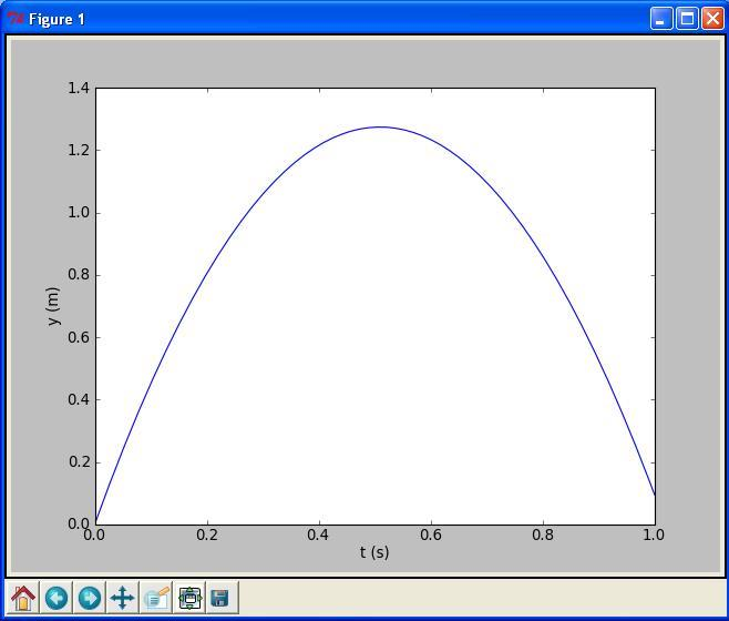
Plot generated by the script ball_plot.py showing the vertical position of the ball at a thousand points in time
The value returned from linspace (being stored in t) is an array,
i.e., a collection of numbers. When we start computing with this
collection of numbers in the arithmetic expression
v0*t - 0.5*g*t**2, the expression is calculated for
every number in t (i.e., every \(t_i\) for \(i = 0, 1,..., 1000\)), yielding a similar collection of 1001 numbers in the result y. That is, y is also an array.
This technique of computing all numbers “in one chunk” is referred to
as vectorization. When it can be used, it is very handy, since both
the amount of code and computation time is reduced compared to writing
a corresponding for or while loop (the chapter Basic constructions) for doing the same thing.
The plotting commands are simple:
plot(t, y)means plotting all theycoordinates versus all thetcoordinatesxlabel('t (s)')places the textt (s)on the \(x\) axisylabel('y (m)')places the texty (m)on the \(y\) axis
At this stage, you are strongly encouraged to do Exercise 4: Volumes of three cubes. It builds on the example above, but is much simpler both with respect to the mathematics and the amount of numbers involved.
More basic concepts
So far we have seen a few basic examples on how to apply Python programming to solve mathematical problems. Before we can go on with other and more realistic examples, we need to briefly treat some topics that will be frequently required in later chapters. These topics include computer science concepts like variables, objects, error messages, and warnings; more numerical concepts like rounding errors, arithmetic operator precedence, and integer division; in addition to more Python functionality when working with arrays, plotting, and printing.
Using Python interactively
Python can also be used interactively. That is, we do not first write
a program in a file and execute it, but we give statements and
expressions to what is known as a Python shell. We recommend to use
IPython as shell (because it is superior to alternative Python
shells). With Spyder, Ipython is available at startup, appearing
as the lower right window. Following the IPython prompt In [1]: (a
prompt means a “ready sign”, i.e. the program allows you to enter
a command, and different programs often have different looking
prompts), you may do calculations:
In  [1]: 2+2
Out [1]: 4

In  [2]: 2*3
Out [2]: 6

In  [3]: 10/2
Out [3]: 5

In  [4]: 2**3
Out [4]: 8
The response from IPython is preceded by Out [q]:,
where q equals p when the response is to input “number” p.
Note that, as in a program, you may have to use import before using
pi or functions like sin, cos, etc. That is, at the prompt, do
the command from math import * before you use pi or sin,
etc. Importing other modules than math may be relevant, depending on
what your aim is with the computations.
You may also define variables and use formulas interactively as
In [1]: v0 = 5

In [2]: g = 9.81

In [3]: t = 0.6

In [4]: y = v0*t - 0.5*g*t**2

In [5]: print y
------> print(y)
1.2342
Sometimes you would like to repeat a command you have given earlier, or perhaps give a command that is almost the same as an earlier one. Then you can use the up-arrow key. Pressing this one time gives you the previous command, pressing two times gives you the command before that, and so on. With the down-arrow key you can go forward again. When you have the relevant command at the prompt, you may edit it before pressing enter (which lets Python read it and take action).
Arithmetics, parentheses and rounding errors
When the arithmetic operators +, -, *, / and
** appear in an expression, Python gives them a certain
precedence. Python interprets the expression from left to right,
taking one term (part of expression between two successive + or -)
at a time. Within each term, **
is done before * and /. Consider
the expression
x = 1*5**2 + 10*3 - 1.0/4.
There are three terms here
and interpreting this, Python starts from the left. In the first term,
1*5**2,
it first does 5**2 which equals 25. This is then
multiplied by 1 to give 25 again. The second term is 10*3, i.e.,
30. So the first two terms add up to 55. The last term gives 0.25, so
the final result is 54.75 which becomes the value of x.
Note that parentheses are often very important to group parts of
expressions together in the intended way. Let us say x = 4 and that
you want to divide 1.0 by x + 1. We know the answer is 0.2, but the
way we present the task to Python is critical, as shown by the
following example.
In [1]: x = 4

In  [2]: 1.0/x+1
Out [2]: 1.25

In  [3]: 1.0/(x+1)
Out [3]: 0.20000000000000001
In the first try, we see that 1.0 is divided by x (i.e., 4), giving
0.25, which is then added to 1. Python did not understand that our
complete denominator was x+1. In our second try, we used parentheses
to “group” the denominator, and we got what we wanted. That is,
almost what we wanted! Since most numbers can be represented only
approximately on the computer, this gives rise to what is called
rounding errors. We should have got 0.2 as our answer, but the
inexact number representation gave a small error. Usually, such errors
are so small compared to the other numbers of the calculation, that we
do not need to bother with them. Still, keep it in mind, since you
will encounter this issue from time to time. More details regarding number
representations on a computer is given in the section Finite precision of floating-point numbers.
Variables and objects
Variables in Python will be of a certain type. If you have an
integer, say you have written x = 2 in some Python program, then x
becomes an integer variable, i.e., a variable of type
int. Similarly, with the statement x = 2.0, x becomes a float
variable (the word float is just computer language for a real
number). In any case, Python thinks of x as an object, of type int
or float. Another common type of variable is str, i.e. a string,
needed when you want to store text. When Python interprets x = "This
is a string", it stores the text (in between the quotes) in the
variable x. This variable is then an object of type str. You may
convert between variable types if it makes sense. If, e.g., x is an
int object, writing y = float(x) will make y a floating point
representation of x. Similarly, you may write int(x) to produce an
int if x is originally of type float. Type conversion may also occur
automatically, as shown just below.
Names of variables should be chosen so that they are descriptive. When
computing a mathematical quantity that has some standard symbol,
e.g. \(\alpha\), this should be reflected in the name by letting the
word alpha be part of the name for the corresponding variable in the
program. If you, e.g., have a variable for counting the number of
sheep, then one appropriate name could be no_of_sheep. Such naming
makes it much easier for a human to understand the written
code. Variable names may also contain any digit from 0 to 9, or
underscores, but can not start with a digit. Letters may be lower or
upper case, which to Python is different. Note that certain names in
Python are reserved, meaning that you can not use these as names for
variables. Some examples are for, while, if, else, global,
return and elif. If you accidentally use a reserved word as a
variable name you get an error message.
We have seen that, e.g., x = 2 will assign the value 2 to the
variable x. But how do we write it if we want to increase x by 4?
We may write an assignment like x = x + 4, or (giving a faster
computation) x += 4. Now Python interprets this as: take whatever
value that is in x, add 4, and let the result become the new value
of x. In other words, the old value of x is used on the right
hand side of =, no matter how messy the expression might be, and the
result becomes the new value of x. In a similar way, x -= 4
reduces the value of x by 4, x *= 4 multiplies x by 4, and x /=
4 divides x by 4, updating the value of x accordingly.
What if x = 2, i.e., an object of type int, and we add 4.0, i.e., a
float? Then automatic type conversion takes place, and the new x
will have the value 6.0, i.e., an object of type float as seen here,
In  [1]: x = 2

In  [2]: x = x + 4.0

In  [3]: x
Out [3]: 6.0
Note that Python programmers, and Python (in printouts), often write, e.g., \(2.\) which by definition is the integer \(2\) represented as a float.
Integer division
Another issue that is important to be aware of is integer division. Let us look at a small example, assuming we want to divide one by four.
In  [1]: 1/4
Out [1]: 0

In  [2]: 1.0/4
Out [2]: 0.25
We see two alternative ways of writing it, but only the last way of writing it gave the correct (i.e., expected) result! Why?
With Python version 2, the first alternative gives what is called
integer division, i.e., all decimals in the answer are disregarded,
so the result is rounded down to the nearest integer. To avoid it, we
may introduce an explicit decimal point in either the numerator, the
denominator, or in both. If you are new to programming, this is
certainly strange behavior. However, you will find the same feature in
many programming languages, not only Python, but actually all languages
with significant inheritance from C. If your numerator or denominator
is a variable, say you have 1/x, you may write 1/float(x) to be on
safe grounds.
Python version 3 implements mathematical real number division by /
and requires the operator // for integer division (// is also
available in Python version 2). Although Python version 3 eliminates
the problems with unintended integer division, it is important to know
about integer division when doing computing in most other languages.
Formatting text and numbers
Results from scientific computations are often to be reported
as a mixture of text and numbers. Usually, we want to control
how numbers are formatted. For example, we may want to write 1/3
as 0.33 or 3.3333e-01 (\(3.3333\cdot 10^{-1}\)).
The print command is the key
tool to write out text and numbers with full control of
the formatting. The first argument to print
is a string with a particular syntax to specify the formatting, the
so-called printf syntax. (The peculiar name stems from the printf
function in the programming language C where the syntax was first
introduced.)
Suppose we have a real number 12.89643, an integer 42, and
a text 'some message' that we want to write out in
the following two alternative ways:
real=12.896, integer=42, string=some message
real=1.290e+01, integer=   42, string=some message
The real number is first written in decimal notation with three
decimals, as 12.896, but afterwards in scientific notation
as 1.290e+01. The integer is first written as compactly as
possible, while on the second line, 42 is formatted in a
text field of width equal to five characters.
The following program, formatted_print.py, applies the printf syntax to control the formatting displayed above:
real = 12.89643
integer = 42
string = 'some message'
print 'real=%.3f, integer=%d, string=%s' % (real, integer, string)
print 'real=%9.3e, integer=%5d, string=%s' % (real, integer, string)
The output of print is a string,
specified in terms of text and a set of variables to be inserted in the text.
Variables are inserted in the text at places indicated by %.
After % comes a specification of the formatting, e.g, %f
(real number), %d (integer), or %s (string).
The format %9.3f means a real number in decimal notation, with
3 decimals, written in a field of width equal to 9 characters.
The variant %.3f means that the number is written as compactly as
possible, in decimal notation, with three decimals. Switching
f with e or E results in the scientific notation, here
1.290e+01 or 1.290E+01. Writing %5d means that an integer
is to be written in a field of width equal to 5 characters.
Real numbers can also be specified with %g, which is used
to automatically choose between decimal or scientific
notation, from what gives the most compact output
(typically, scientific notation is appropriate for very small and very large numbers
and decimal notation for the intermediate range).
A typical example of when printf formatting is required, arises when nicely aligned columns of numbers are to be printed. Suppose we want to print a column of \(t\) values together with associated function values \(g(t)=t\sin(t)\) in a second column. The simplest approach would be
from math import sin

t0 = 2
dt = 0.55

# Unformatted print
t = t0 + 0*dt; g = t*sin(t)
print t, g

t = t0 + 1*dt; g = t*sin(t)
print t, g

t = t0 + 2*dt; g = t*sin(t)
print t, g
with output
2.0 1.81859485365
2.55 1.42209347935
3.1 0.128900053543
(Repeating the same set of statements multiple times, as done above,
is not good programming practice - one should use a for loop, as
explained later in the section For loops.)
Observe that the numbers in the columns
are not nicely aligned. Using the printf syntax
'%6.2f %8.3f' % (t, g) for t and g, we can control the width of each
column and also the number of decimals, such that the numbers
in a column are aligned under each other and
written with the same precision. The output
then becomes
Formatting via printf syntax
  2.00     1.819
  2.55     1.422
  3.10     0.129
We shall frequently use the printf syntax throughout the book so there will be plenty of further examples.
The modern alternative to printf syntax
Modern Python favors the new format string syntax over printf:
print 'At t={t:g} s, y={y:.2f} m'.format(t=t, y=y)
which corresponds to the printf syntax
print 'At t=%g s, y=%.2f m' % (t, y)
The slots where variables are inserted are now recognized by curly
braces, and in format we list the variable names inside curly
braces and their equivalent variables in the program.
Since the printf syntax is so widely used in many programming languages, we stick to that in the present book, but Python programmers will frequently also meet the newer format string syntax, so it is important to be aware its existence.
Arrays
In the program ball_plot.py from the chapter A Python program with vectorization and plotting we saw how
1001 height computations were executed and stored in the variable y,
and then displayed in a plot showing y versus t, i.e., height
versus time. The collection of numbers in y (or t, respectively)
was stored in what is called an array, a construction also found in
most other programming languages. Such arrays are created and
treated according to certain rules, and as a programmer, you may
direct Python to compute and handle arrays as a whole, or as
individual array elements. Let us briefly look at a smaller such
collection of numbers.
Assume that the heights of four family members have been collected. These heights may be generated and stored in an array, e.g., named h, by writing
h = zeros(4)
h[0] = 1.60
h[1] = 1.85
h[2] = 1.75
h[3] = 1.80
where the array elements appear as h[0], h[1], etc. Generally,
when we read or talk about the array elements of some array a, we
refer to them by reading or saying “a of zero” (i.e., a[0]), “a of
one” (i.e., a[1]), and so on. The very first line in the example
above, i.e.
h = zeros(4)
instructs Python to reserve, or allocate, space in memory for an
array h with four elements and initial values set to 0.
The next four lines overwrite the zeros
with the desired numbers (measured heights), one number for each
element. Elements are, by rule, indexed (numbers within brackets)
from 0 to the last element, in this case 3. We say that Python has
zero based indexing. This differs from one based indexing (e.g.,
found in Matlab) where the array index starts with 1.
As illustrated in the code, you may refer to the array as a whole by
the name h, but also to each individual element by use of the
index. The array elements may enter in computations as individual
variables, e.g., writing
z = h[0] + h[1] + h[2] + h[3] will compute
the sum of all the elements in h, while the result is assigned to
the variable z. Note that this way of creating an array is a bit
different from the one with linspace, where the filling in of
numbers occurred automatically “behind the scene”.
By the use of a colon, you may pick out a slice of an array. For
example, to create a new array from the two elements h[1] and
h[2], we could write slice_h = h[1:3]. Note that the index
specification 1:3 means indices 1 and 2, i.e., the last index is
not included. For the generated slice_h array, indices are as usual,
i.e., 0 and 1 in this case. The very last entry in an array may be
addressed as, e.g., h[-1].
Copying arrays requires some care since simply writing new_h = h
will, when you afterwards change elements of new_h, also change the
corresponding elements in h! That is, h[1] is also changed when
writing
new_h = h
new_h[1] = 5.0
print h[1]
In this case we do not get \(1.85\) out on the screen, but \(5.0\). To
really get a copy that is decoupled from the original array, you may
write new_h = copy(h). However, copying a slice works
straightforwardly (as shown above), i.e. an explicit use of copy is not
required.
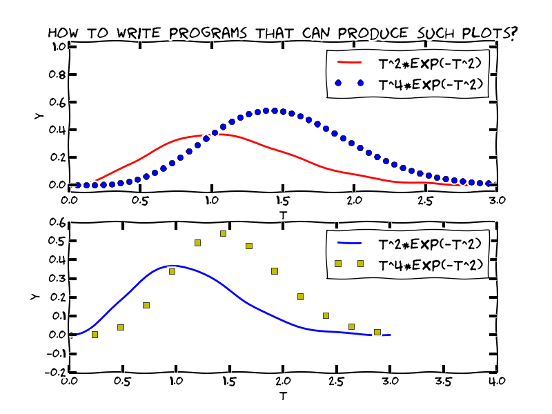
Plotting
Sometimes you would like to have two or more curves or graphs in
the same plot. Assume we have h as above, and also an array H with
the heights \(0.50\) m, \(0.70\) m, \(1.90\) m,
and \(1.75\) m from a family next door. This may be done with the
program
plot_heights.py
given as
from numpy import zeros
import matplotlib.pyplot as plt

h = zeros(4)
h[0] = 1.60; h[1] = 1.85; h[2] = 1.75; h[3] = 1.80
H = zeros(4)
H[0] = 0.50; H[1] = 0.70; H[2] = 1.90; H[3] = 1.75

family_member_no = zeros(4)
family_member_no[0] = 0; family_member_no[1] = 1
family_member_no[2] = 2; family_member_no[3] = 3

plt.plot(family_member_no, h, family_member_no, H)
plt.xlabel('Family member number')
plt.ylabel('Height (m)')
plt.show()
Running the program gives the plot shown in Figure Generated plot for the heights of family members from two families.
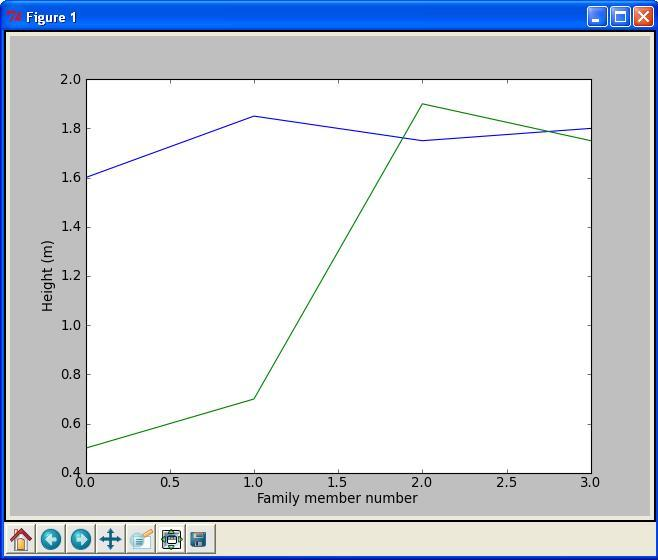
Generated plot for the heights of family members from two families
Alternatively, the two curves could have been plotted in the same plot by use of two plot commands, which gives more freedom as to how the curves appear. To do this, you could plot the first curve by
plot(family_member_no, h)
hold('on')
Then you could (in principle) do a lot of other things in your code, before you plot the second curve by
plot(family_member_no, H)
hold('off')
Notice the use of hold here. hold('on') tells Python
to plot also the following curve(s) in the same window.
Python does so until it reads hold('off'). If you do not use the
hold('on') or hold('off') command,
the second plot command will overwrite the first one, i.e.,
you get only the second curve.
In case you would like the two curves plotted in two separate plots, you can do this by plotting the first curve straightforwardly with
plot(family_member_no, h)
then do other things in your code, before you do
figure()
plot(family_member_no, H)
Note how the graphs are made continuous by Python, drawing straight
lines between the four data points of each family. This is the
standard way of doing it and was also done when plotting our 1001
height computations with ball_plot.py in the chapter A Python program with vectorization and plotting. However, since there were so many data points then, the
curve looked nice and smooth. If preferred, one may also plot only the
data points. For example, writing
plot(h, '*')
will mark only the data points with the star symbol. Other symbols like circles etc. may be used as well.
There are many possibilities in Python for adding information to a plot or for changing its appearance. For example, you may add a legend by the instruction
legend('This is some legend')
or you may add a title by
title('This is some title')
The command
axis([xmin, xmax, ymin, ymax])
will define the plotting range for the \(x\) axis to stretch from
xmin to xmax and, similarly, the plotting range for the
\(y\) axis from ymin to ymax.
Saving the figure to file is achieved by the command
savefig('some_plot.png')   # PNG format
savefig('some_plot.pdf')   # PDF format
savefig('some_plot.gif')   # GIF format
savefig('some_plot.eps')   # Encanspulated PostScript format
For the reader who is into linear algebra, it may be useful to know that standard matrix/vector operations are straightforward with arrays, e.g., matrix-vector multiplication.
What is needed though, is
to create the right variable types (after having imported an appropriate module). For example, assume you would like to calculate the vector \(\bf{y}\) (note that boldface is used for vectors and matrices) as \(\bf{y} = \bf{Ax}\), where \(\bf{A}\) is a \(2 \times 2\) matrix and \(\bf{x}\) is a vector. We may do this as illustrated by the program matrix_vector_product.py reading
from numpy import zeros, mat, transpose

x = zeros(2)
x = mat(x)
x = transpose(x)
x[0] = 3;   x[1] = 2   # Pick some values

A = zeros((2,2))
A = mat(A)
A[0,0] = 1;  A[0,1] = 0
A[1,0] = 0;  A[1,1] = 1

# The following gives y = x since A = I, the identity matrix
y = A*x
print y
Here, x is first created as an array, just as we did above. Then
the variable type of x is changed to mat, i.e., matrix, by the
line x = mat(x). This is followed by a transpose of x from
dimension \(1 \times 2\) (the default dimension) to \(2 \times 1\) with
the statement x = transpose(x), before some test values are plugged
in. The matrix A is first created as a two dimensional array with A
= zeros((2,2)) before conversion and filling in values take
place. Finally, the multiplication is performed as y = A*x. Note the
number of parentheses when creating the two dimensional array
A. Running the program gives the following output on the screen:
[[3.]
 [2.]]
Error messages and warnings
All programmers experience error messages, and usually to a large extent during the early learning process. Sometimes error messages are understandable, sometimes they are not. Anyway, it is important to get used to them. One idea is to start with a program that initially is working, and then deliberately introduce errors in it, one by one. (But remember to take a copy of the original working code!) For each error, you try to run the program to see what Python’s response is. Then you know what the problem is and understand what the error message is about. This will greatly help you when you get a similar error message or warning later.
Very often, you will experience that there are errors in the program you have written. This is normal, but frustrating in the beginning. You then have to find the problem, try to fix it, and then run the program again. Typically, you fix one error just to experience that another error is waiting around the corner. However, after some time you start to avoid the most common beginner’s errors, and things run more smoothly. The process of finding and fixing errors, called debugging, is very important to learn. There are different ways of doing it too.
A special program (debugger) may be used to help you check (and
do) different things in the program you need to fix. A simpler
procedure, that often brings you a long way, is to print information
to the screen from different places in the program. First of all, this
is something you should do (several times) during program development
anyway, so that things get checked as you go along. However, if the
final program still ends up with error messages, you may save a copy
of it, and do some testing on the copy. Useful testing may then be to
remove, e.g., the latter half of the program (by inserting comment
signs #), and insert print commands at clever places to see what is
the case. When the first half looks ok, insert parts of what was
removed and repeat the process with the new code. Using simple numbers
and doing this in parallel with hand calculations on a piece of paper
(for comparison) is often a very good idea.
Python also offers means to detect and handle errors by the program
itself! The programmer must then foresee (when writing the code) that
there is a potential for error at some particular point. If, for
example, some user of the program is asked (by the running program) to
provide a number, and intends to give the number 5, but instead writes
the word five, the program could run into trouble. A
try-exception construction may be used by
the programmer to check for such errors and act appropriately (see
the chapter Newton’s method for an example), avoiding a program
crash. This procedure of trying an action and then recovering from
trouble, if necessary, is referred to as exception handling and
is the modern way of dealing with errors in a program.
When a program finally runs without error messages, it might be tempting to think that Ah..., I am finished!. But no! Then comes program testing, you need to verify that the program does the computations as planned. This is almost an art and may take more time than to develop the program, but the program is useless unless you have much evidence showing that the computations are correct. Also, having a set of (automatic) tests saves huge amounts of time when you further develop the program.
Verification versus validation
Verification is important, but validation is equally important. It is great if your program can do the calculations according to the plan, but is it the right plan? Put otherwise, you need to check that the computations run correctly according to the formula you have chosen/derived. This is verification: doing the things right. Thereafter, you must also check whether the formula you have chosen/derived is the right formula for the case you are investigating. This is validation: doing the right things. In the present book, it is beyond scope to question how well the mathematical models describe a given phenomenon in nature or engineering, as the answer usually involves extensive knowledge of the application area. We will therefore limit our testing to the verification part.
Input data
Computer programs need a set of input data and the purpose is to use these data to compute output data, i.e., results. In the previous program we have specified input data in terms of variables. However, one often wants to get the input through some dialog with the user. Here is one example where the program asks a question, and the user provides an answer by typing on the keyboard:
age = input('What is your age? ')
print "Ok, so you're half way to %d, wow!" % (age*2)
So, after having interpreted and run the first line, Python has
established the variable age and assigned your input to it. The
second line combines the calculation of twice the age with a message
printed on the screen. Try these two lines in a little test program to
see for yourself how it works.
The input function is useful for numbers, lists (the chapter Basic constructions),
and tuples (the chapter Basic constructions).
For pure text, the user must either enclose the input in quotes, or the program must use
the raw_input function instead:
name = raw_input('What is your name? ')
There are other ways of providing input to a program as well, e.g., via a graphical interface (as many readers will be used to) or at the command line (i.e., as parameters succeeding, on the same line, the command that starts the program). Reading data from a file is yet another way. Logically, what the program produces when run, e.g. a plot or printout to the screen or a file, is referred to as program output.
Symbolic computations
Even though the main focus in this book is programming of numerical methods, there are occasions where symbolic (also called exact or analytical) operations are useful. Doing symbolic computations means, as the name suggests, that we do computations with the symbols themselves rather than with the numerical values they could represent. Let us illustrate the difference between symbolic and numerical computations with a little example. A numerical computation could be
x = 2
y = 3
z = x*y
print z
which will make the number 6 appear on the screen. A symbolic counterpart of this code could be
from sympy import *
x, y = symbols('x y')
z = x*y
print z
which causes the symbolic result x*y to appear on the screen.
Note that no numerical value was assigned to any of the variables
in the symbolic computation. Only the symbols were used, as when
you do symbolic mathematics by hand on a piece of paper.
Symbolic computations in Python make use of the
SymPy package.
Each symbol is represented
by a standard variable, but the name of the symbol must be
declared with Symbol(name) for a single symbol, or symbols(name1 name2 ...) for multiple symbols..
The following script
example_symbolic.py
is a quick demonstration
of some of the basic symbolic operations that are supported in Python.
from sympy import *

x = Symbol('x')
y = Symbol('y')

print 2*x + 3*x - y                # Algebraic computation
print diff(x**2, x)                # Differentiates x**2 wrt. x
print integrate(cos(x), x)         # Integrates cos(x) wrt. x
print simplify((x**2 + x**3)/x**2) # Simplifies expression
print limit(sin(x)/x, x, 0)        # Finds limit of sin(x)/x as x->0
print solve(5*x - 15, x)           # Solves 5*x = 15
Other symbolic calculations like Taylor series expansion, linear algebra (with matrix and vector operations), and (some) differential equation solving are also possible.
Symbolic computations are also readily accessible through the (partly) free
online tool WolframAlpha, which
applies the very advanced Mathematica package as symbolic engine.
The disadvantage with WolframAlpha compared to the
SymPy package is that the results cannot
automatically be imported into your code and used for further
analysis. On the other hand, WolframAlpha has the advantage that it
displays many additional mathematical results related to the given
problem. For example, if we type 2x + 3x - y in WolframAlpha, it
not only simplifies the expression to 5x - y, but it also makes plots
of the function \(f(x,y)=5x-y\), solves the equation \(5x - y = 0\), and
calculates the integral \(\int\int(5x+y)dxdy\). The commercial Pro
version can also show a step-by-step of the analytical computations in
the problem. You are strongly encouraged to try out these commands in
WolframAlpha:
diff(x^2, x)ordiff(x**2, x)integrate(cos(x), x)simplify((x**2 + x**3)/x**2)limit(sin(x)/x, x, 0)solve(5*x - 15, x)
WolframAlpha is very flexible with respect to syntax.
Another impressive tool for symbolic computations is Sage, which is a very comprehensive package with the aim of “creating a viable free open source alternative to Magma, Maple, Mathematica and Matlab”. Sage is implemented in Python. Projects with extensive symbolic computations will certainly benefit from exploring Sage.
Concluding remarks
Programming demands you to be accurate
In this chapter, you have seen some examples of how simple things may
be done in Python. Hopefully, you have tried to do the examples on
your own. If you have, most certainly you have discovered that what
you write in the code has to be very accurate. For example, with our
previous example of four heights collected in an array h, writing
h(0) instead of h[0]
gives an error, even if you and I know
perfectly well what you mean! Remember that it is not a human that
runs your code, it is a machine. Therefore, even if the meaning of
your code looks fine to a human eye, it still has to comply in detail
to the rules of the programming language. If not, you get warnings and
error messages. This also goes for lower and upper case letters.
If you do from math import * and give the command pi, you get
\(3.1415\ldots\). However, if you write Pi, you get an error
message.
Pay attention to such details also when they are given in later chapters.
Fast code versus readable and correct code
Numerical computing has a strong tradition in paying much attention to creating fast code. Real industrial applications of numerical computing often involves simulations that run for hours, days, and even weeks. Fast code is tremendously important in those cases. The problem with a strong focus on fast code, unfortunately, is sometimes that clear and easily understandable constructions are replaced by clever and less readable, but faster code. However, for beginners it is most important to learn to write readable and correct code. We will make some comments on constructions that are fast or slow, but the main focus of this book is to teach how to write correct programs, not the fastest possible programs.
Deleting data no longer in use
Python has automatic garbage collection, meaning that there is no need to delete variables (or objects) that are no longer in use. Python takes care of this by itself. This is opposed to, e.g., Matlab, where explicit deleting sometimes may be required.
Tip: how to deal with long lines
If a statement in a program gets too long, it may be continued on the next line by inserting a back-slash at the end of the line before proceeding on the next line. However, no blanks must occur after the back-slash!
The present introductory book just provides a tiny bit of all the functionality that Python has to offer. An important source of information is the official Python documentation website (http://docs.python.org/), which provides a Python tutorial, the Python Library Reference, a Language Reference, and more. Several excellent books are also available (http://wiki.python.org/moin/PythonBooks), but not so many with a scientific computing focus. One exception is Langtangen’s comprehensive book A Primer on Scientific Programming with Python, Springer, 2016.
Exercises
Exercise 1: Error messages
Save a copy of the program ball.py and confirm that the copy runs as the
original. You are now supposed to introduce errors in the code, one by
one. For each error introduced, save and run the program, and comment
how well Python’s response corresponds to the actual error. When you
are finished with one error, re-set the program to correct behavior
(and check that it works!) before moving on to the next error.
a)
Insert the word hello on the empty line above the assignment to v0.
Solution. An error message is printed, which at the end states that
NameError: name 'hello' is not defined
The error message tells us explicitly what is wrong.
b)
Remove the # sign in front of the
comment initial velocity.
Solution. An error message is printed, which states that
    v0 = 5   initial velocity
SyntaxError: invalid syntax
Python repeats the particular code line where the problem is. Then, it tells us that there is a syntax error in this line. It is up to the programmer to find the syntax error in the line.
c)
Remove the = sign in the assignment to v0.
Solution. An error message is printed, which at the end states that
    v0  5   #initial velocity
SyntaxError: invalid syntax
Python repeats the particular code line where the problem is. Then, it tells us that there is a syntax error in this line. It is up to the programmer to find the syntax error in the line.
d)
Change the reserved word print into pint.
Solution. An error message is printed, which at the end states that
    pint y
SyntaxError: invalid syntax
Python repeats the particular code line where the problem is. Then, it tells us that there is a syntax error in this line. It is up to the programmer to find the syntax error in the line.
e)
Change the calculation of y to y = v0*t.
Solution.
We get no error message this time, even if the calculation of y
is wrong! This is because, to Python, the “new” way of calculating
y is perfectly legal, and Python can not know what we wanted to
compute. This is therefore another kind of error that sometimes may
be hard to find, since we get no error message. To find such errors,
answers have to be analyzed quantitatively in some way.
f)
Change the line print y to print x.
Solution. An error message is printed, which at the end states that
    print x
NameError: name 'x' is not defined
Python repeats the particular code line
where the problem is. Then, it explicitly tells us the problem,
namely that x is not defined.
g) Replace the statement
y = v0*t - 0.5*g*t**2
by
y = v0*t - (1/2)*g*t**2
Solution.
We get no error message, but the wrong answer 3 (instead of 1.2342).
The problem is that 1/2 is an integer divison that rounds to zero, so
the computation now becomes equivalent to y = v0*t, which is wrong.
Filename: testing_ball.py.
Exercise 2: Volume of a cube
Write a program that computes the volume \(V\) of a cube with sides of length \(L = 4\) cm and prints the result to the screen. Both \(V\) and \(L\) should be defined as separate variables in the program. Run the program and confirm that the correct result is printed.
Hint.
See ball.py in the text.
Solution. The code reads:
L = 4       # i.e., in cm
V = L**3
print "The volume is: ", V
Running the program gives the output
The volume is: 64
Filename: cube_volume.py.
Exercise 3: Area and circumference of a circle
Write a program that computes both the circumference \(C\) and the area \(A\) of a circle with radius \(r = 2\) cm. Let the results be printed to the screen on a single line with an appropriate text. The variables \(C\), \(A\) and \(r\) should all be defined as a separate variables in the program. Run the program and confirm that the correct results are printed.
Solution. The code reads:
from math import *

r = 2
C = 2*pi*r
A = pi*r**2

print "Circumference: %g, Area: %g" % (C, A)
Running the program gives the output
Circumference: 12.5664, Area: 12.5664
Filename: circumference_and_area.py.
Exercise 4: Volumes of three cubes
We are interested in the volume \(V\) of a cube with length \(L\): \(V=L^3\), computed for three different values of \(L\).
a)
Use the linspace function to compute three values
of \(L\), equally spaced on the interval \([1,3]\).
Solution.
We must remember to import the function linspace before we can use it.
In [1]: from numpy import linspace
In [2]: linspace(1, 3, 3)
Out [2]: array([1., 2., 3.])
b) Carry out by hand the computation \(V=L^3\) if \(L\) is an array with three elements. That is, compute \(V\) for each value of \(L\).
Solution. You should get 1, 8 and 27, which afterwards should compare favorably to output from the code.
c)
In a program, write out the result V of V = L**3
when L is an array with three elements as computed by linspace in a).
Compare the resulting volumes with your hand calculations.
Solution. The code reads:
from numpy import *

L = linspace(1, 3, 3)
V = L**3
print "Volumes:", V
Running the program gives the printout
Volumes: [ 1. 8. 27. ]
d)
Make a plot of V versus L.
Solution. The code reads:
from matplotlib.pyplot import *
plot(L, V)
xlabel('Length of side')
ylabel('Volume')
The plot looks like
Remark. Observe that straight lines are drawn between the three points. To make a smoother cubic curve \(V=L^3\), we would need to compute more \(L\) and \(V\) values on the curve.
Filename: volume3cubes.py.
Exercise 5: Average of integers
Write a program that stores the sum \(1+2+3+4+5\) in one variable and then creates another variable with the average of these five numbers. Print the average to the screen and check that the result is correct.
Solution. The code reads:
sum = 1 + 2 + 3 + 4 + 5
average = sum/5.0
print "average: ", average
Running the program gives
average: 3.0
Filename: average_int.py.
Exercise 6: Interactive computing of volume and area
a) Compute the volume in Exercise 2: Volume of a cube by using Python interactively, i.e., do the computations at the command prompt (in a Python shell as we also say). Compare with what you got previously from the written program.
Solution.
In [1]: L = 4
In [2]: V = L**3
In [3]: print "The volume is: ", V
The volume is: 64
b) Do the same also for Exercise 3: Area and circumference of a circle.
Solution.
from math import *
In [1]: r = 2
In [2]: C = 2*pi*r
In [3]: A = pi*r**2
In [4]: print "Circumference: %g, Area: %g " % (C,A)
Circumference: 12.5664, Area: 12.5664
Exercise 7: Peculiar results from division
Consider the following interactive Python session:
In [1]: x=2; y=4

In [2]: x/y
Out[2]: 0
What is the problem and how can you fix it?
Solution.
Because of integer division Python will round this to zero
(since the numerator is smaller than the denominator). The problem
may be fixed by using the function float either in the numerator or
in the denominator (or in both places). If we use float in the numerator,
the code line with the division reads:
In [2]: float(x)/y
The answer then correctly becomes \(0.5\).
Exercise 8: Update variable at command prompt
Invoke Python interactively and perform the following steps.
- Initialize a variable
xto 2. - Add 3 to
x. Print out the result. - Print out the result of
x + 1*2and(x+1)*2. (Observe how parentheses make a difference). - What variable type is
x?
Solution.
In [1]: x = 2
In [2]: x += 3
In [3]: print x + 1*2
7
In [4]: print (x + 1)*2
12
In [5]: type(x)
Out [5]: int
Exercise 9: Formatted print to screen
Write a program that defines two variables as x = pi and y = 2.
Then let the program compute the product z of these two variables
and print the result to the screen as
Multiplying 3.14159 and 2 gives 6.283
Solution. The code reads:
from math import pi

x = pi
y = 2
z = x*y

print "Multiplying %g and %g gives %g" % (x, y, z)
Running the program prints the requested output.
Filename: formatted_print.py.
Exercise 10: Python documentation and random numbers
Write a program that prints four random to the screen. The numbers should be drawn from a uniform distribution over the interval \([0,10)\) (0 inclusive, 10 exclusive). Find the information needed for the task, see for example http://docs.python.org.
Hint.
Python has a module random that contains a function by the name uniform.
Solution. The code reads:
import random
print random.uniform(0, 10)
print random.uniform(0, 10)
print random.uniform(0, 10)
print random.uniform(0, 10)
Running the program gives for example (note that numbers change when you run the program again)
7.04892469523
4.64465984386
8.46022195385
0.458184395321
Filename: drawing_random_numbers.py.

Remember to insert comments to explain your code
When you write a computer program, you have two very different kinds of readers. One is Python, which will interpret and run your program according to the rules. The other is some human, for example, yourself or a peer. It is very important to organize and comment the code so that you can go back to your own code after, e.g., a year and still understand what clever constructions you put in there. This is relevant when you need to change or extend your code (which usually happens often in reality). Organized coding and good commenting is even more critical if other people are supposed to understand code that you have written.