Basic constructions

If tests, colon and indentation

Very often in life, and in computer programs, the next action depends on the outcome of a question starting with “if”. This gives the possibility to branch into different types of action depending on some criterion. Let us as usual focus on a specific example, which is the core of so-called random walk algorithms used in a wide range of branches in science and engineering, including materials manufacturing and brain research. The action is to move randomly to the north (N), east (E), south (S), or west (W) with the same probability. How can we implement such an action in life and in a computer program?

We need to randomly draw one out of four numbers to select the direction in which to move. A deck of cards can be used in practice for this purpose. Let the four suits correspond to the four directions: clubs to N, diamonds to E, hearts to S, and spades to W, for instance. We draw a card, perform the corresponding move, and repeat the process a large number of times. The resulting path is a typical realization of the path of a diffusing molecule.

In a computer program, we need to draw a random number, and depending on the number, update the coordinates of the point to be moved. There are many ways to draw random numbers and translate them into (e.g.) four random directions, but the technical details usually depend on the programming language. Our technique here is universal: we draw a random number in the interval \([0,1)\) and let \([0,0.25)\) correspond to N, \([0.25,0.5)\) to E, \([0.5,0.75)\) to S, and \([0.75,1)\) to W. Let x and y hold the coordinates of a point and let d be the length of the move. A pseudo code (i.e., not “real” code, just a “sketch of the logic”) then goes like

r = random number in [0,1)
if 0 <= r < 0.25
   move north: y = y + d
else if 0.25 <= r < 0.5
   move east:  x = x + d
else if 0.5 <= r < 0.75
   move south:  y = y - d
else if 0.75 <= r < 1
   move west:  x = x - d

Note the need for first asking about the value of r and then performing an action. If the answer to the “if” question is positive (true), we are done and can skip the next else if questions. If the answer is negative (false), we proceed with the next question. The last test if \(0.75\leq r < 1\) could also read just else, since we here cover all the remaining possible r values.

The exact code in Python reads

import random
r = random.random()        # random number in [0,1)
if 0 <= r < 0.25:
   # move north
   y = y + d
elif 0.25 <= r < 0.5:
   # move east
   x = x + d
elif 0.5 <= r < 0.75:
   # move south
   y = y - d
else:
   # move west
   x = x - d

We use else in the last test to cover the different types of syntax that is allowed. Python recognizes the reserved words if, elif (short for else if), and else and expects the code to be compatible with the rules of if tests:

• The test reads if condition:, elif condition:, or else:, where condition is a boolean expression that evaluates to True or False. Note the closing colon (easy to forget!).
• If condition is True, the following indented block of statements are executed and the remaining if, elif, or else branches are skipped.
• If condition is False, the program flow jumps to the next if, elif, or else branch.

The blocks after if, elif, or else may contain new if tests, if desired. Regarding colon and indent, you will see below that these are required in several other programming constructions as well.

Working with if tests requires mastering boolean expressions. Here are some basic boolean expressions involving the logical operators ==, !=, <, <=, >, and >=. Given the assignment to temp, you should go through each boolean expression below and determine if it is true or false.

temp = 21       # assign value to a variable
temp == 20      # temp equal to 20
temp != 20      # temp not equal to 20
temp <  20      # temp less than 20
temp >  20      # temp greater than 20
temp <= 20      # temp less than or equal to 20
temp >= 20      # temp greater than or equal to 20

Functions

Functions are widely used in programming and is a concept that needs to be mastered. In the simplest case, a function in a program is much like a mathematical function: some input number \(x\) is transformed to some output number. One example is the \(\tanh^{-1}(x)\) function, called atan in computer code: it takes one real number as input and returns another number. Functions in Python are more general and can take a series of variables as input and return one or more variables, or simply nothing. The purpose of functions is two-fold:

1. to group statements into separate units of code lines that naturally belong together (a strategy which may dramatically ease the problem solving process), and/or
2. to parameterize a set of statements such that they can be written only once and easily be re-executed with variations.

Examples will be given to illustrate how functions can be written in various contexts.

If we modify the program ball.py from the chapter A Python program with variables slightly, and include a function, we could let this be a new program ball_function.py as

def y(t):
    v0 = 5                    # Initial velocity
    g = 9.81                  # Acceleration of gravity
    return v0*t - 0.5*g*t**2

time = 0.6       # Just pick one point in time
print y(time)
time = 0.9       # Pick another point in time
print y(time)

When Python reads and interprets this program from the top, it takes the code from the line with def, to the line with return, to be the definition of a function with the name y (note colon and indentation). The return statement of the function y, i.e.

return v0*t - 0.5*g*t**2

will be understood by Python as first compute the expression, then send the result back (i.e., return) to where the function was called from. Both def and return are reserved words. The function depends on t, i.e., one variable (or we say that it takes one argument or input parameter), the value of which must be provided when the function is called.

What actually happens when Python meets this code? The def line just tells Python that here is a function with name y and it has one argument t. Python does not look into the function at this stage (except that it checks the code for syntax errors). When Python later on meets the statement print y(time), it recognizes a function call y(time) and recalls that there is a function y defined with one argument. The value of time is then transferred to the y(t) function such that t = time becomes the first action in the y function. Then Python executes one line at a time in the y function. In the final line, the arithmetic expression v0*t - 0.5*g*t**2 is computed, resulting in a number, and this number (or more precisely, the Python object representing the number) replaces the call y(time) in the calling code such that the word print now precedes a number rather than a function call.

Python proceeds with the next line and sets time to a new value. The next print statement triggers a new call to y(t), this time t is set to 0.9, the computations are done line by line in the y function, and the returned result replaces y(time). Instead of writing print y(time), we could alternatively have stored the returned result from the y function in a variable,

h = y(time)
print h

Note that when a function contains if-elif-else constructions, return may be done from within any of the branches. This may be illustrated by the following function containing three return statements:

def check_sign(x):
    if x > 0:
        return 'x is positive'
    elif x < 0:
        return 'x is negative'
    else:
        return 'x is zero'

Remember that only one of the branches is executed for a single call on check_sign, so depending on the number x, the return may take place from any of the three return alternatives.

To return at the end or not

Programmers disagree whether it is a good idea to use return inside a function where you want, or if there should only be one single return statement at the end of the function. The authors of this book emphasize readable code and think that return can be useful in branches as in the example above when the function is short. For longer or more complicated functions, it might be better to have one single return statement. Be prepared for critical comments if you return wherever you want...

An expression you will often encounter when dealing with programming, is main program, or that some code is in main. This is nothing particular to Python, and simply refers to that part of the program which is outside functions. However, note that the def line of functions is counted into main. So, in ball_function.py above, all statements outside the function y are in main, and also the line def y(t):.

A function may take no arguments, or many, in which case they are just listed within the parentheses (following the function name) and separated by a comma. Let us illustrate. Take a slight variation of the ball example and assume that the ball is not thrown straight up, but at an angle, so that two coordinates are needed to specify its position at any time. According to Newton’s laws (when air resistance is negligible), the vertical position is given by \(y(t) = v_{0y}t - 0.5gt^2\) and the horizontal position by \(x(t) = v_{0x}t\). We can include both these expressions in a new version of our program that prints the position of the ball for chosen times. Assume we want to evaluate these expressions at two points in time, \(t = 0.6s\) and \(t = 0.9s\). We can pick some numbers for the initial velocity components v0y and v0x, name the program ball_position.py, and write it for example as

def y(v0y, t):
    g = 9.81                  # Acceleration of gravity
    return v0y*t - 0.5*g*t**2

def x(v0x, t):
    return v0x*t

initial_velocity_x = 2.0
initial_velocity_y = 5.0

time = 0.6       # Just pick one point in time
print x(initial_velocity_x, time), y(initial_velocity_y, time)
time = 0.9       # ... Pick another point in time
print x(initial_velocity_x, time), y(initial_velocity_y, time)

Now we compute and print the two components for the position, for each of the two chosen points in time. Notice how each of the two functions now takes two arguments. Running the program gives the output

1.2  1.2342
1.8  0.52695

A function may also have no return value, in which case we simply drop the return statement, or it may return more than one value. For example, the two functions we just defined could alternatively have been written as one:

def xy(v0x, v0y, t):
    g = 9.81                          # acceleration of gravity
    return v0x*t, v0y*t - 0.5*g*t**2

Notice the two return values which are simply separated by a comma. When calling the function (and printing), arguments must appear in the same order as in the function definition. We would then write

print xy(initial_x_velocity, initial_y_velocity, time)

The two returned values from the function could alternatively have been assigned to variables, e.g., as

x_pos, y_pos = xy(initial_x_velocity, initial_y_velocity, time)

The variables x_pos and y_pos could then have been printed or used in other ways in the code.

There are possibilities for having a variable number of function input and output parameters (using *args and **kwargs constructions for the arguments). However, we do not go further into that topic here.

Variables that are defined inside a function, e.g., g in the last xy function, are local variables. This means they are only known inside the function. Therefore, if you had accidentally used g in some calculation outside the function, you would have got an error message. The variable time is defined outside the function and is therefore a global variable. It is known both outside and inside the function(s). If you define one global and one local variable, both with the same name, the function only sees the local one, so the global variable is not affected by what happens with the local variable of the same name.

The arguments named in the heading of a function definition are by rule local variables inside the function. If you want to change the value of a global variable inside a function, you need to declare the variable as global inside the function. That is, if the global variable was x, we would need to write global x inside the function definition before we let the function change it. After function execution, x would then have a changed value. One should strive to define variables mostly where they are needed and not everywhere.

Another very useful way of handling function parameters in Python, is by defining parameters as keyword arguments. This gives default values to parameters and allows more freedom in function calls, since the order and number of parameters may vary.

Let us illustrate the use of keyword arguments with the function xy. Assume we defined xy as

def xy(t, v0x=0, v0y=0):
    g = 9.81                          # acceleration of gravity
    return v0x*t, v0y*t - 0.5*g*t**2

Here, t is an ordinary or positional argument, whereas v0x and v0y are keyword arguments or named arguments. Generally, there can be many positional arguments and many keyword arguments, but the positional arguments must always be listed before the keyword arguments in function definition. Keyword arguments are given default values, as shown here with v0x and v0y, both having zero as default value. In a script, the function xy may now be called in many different ways. For example,

print xy(0.6)

would make xy perform the computations with t = 0.6 and the default values (i.e zero) of v0x and v0y. The two numbers returned from xy are printed to the screen. If we wanted to use another initial value for v0y, we could, e.g., write

print xy(0.6,v0y=4.0)

which would make xy perform the calculations with t = 0.6, v0x = 0 (i.e. the default value) and v0y = 4.0. When there are several positional arguments, they have to appear in the same order as defined in the function definition, unless we explicitly use the names of these also in the function call. With explicit name specification in the call, any order of parameters is acceptable. To illustrate, we could, e.g., call xy as

print xy(v0y=4.0, v0x=1.0, t=0.6)

In any programming language, it is a good habit to include a little explanation of what the function is doing, unless what is done by the function is obvious, e.g., when having only a few simple code lines. This explanation is called a doc string, which in Python should be placed just at the top of the function. This explanation is meant for a human who wants to understand the code, so it should say something about the purpose of the code and possibly explain the arguments and return values if needed. If we do that with our xy function from above, we may write the first lines of the function as

def xy(v0x, v0y, t):
    """Compute the x and y position of the ball at time t"""

Note that other functions may be called from within other functions, and function input parameters are not required to be numbers. Any object will do, e.g., string variables or other functions.

Functions are straightforwardly passed as arguments to other functions, as illustrated by the following script function_as_argument.py:

def sum_xy(x, y):
    return x + y

def prod_xy(x, y):
    return x*y

def treat_xy(f, x, y):
    return f(x, y)

x = 2;  y = 3
print treat_xy(sum_xy, x, y)
print treat_xy(prod_xy, x, y)

When run, this program first prints the sum of x and y (i.e., 5), and then it prints the product (i.e., 6). We see that treat_xy takes a function name as its first parameter. Inside treat_xy, that function is used to actually call the function that was given as input parameter. Therefore, as shown, we may call treat_xy with either sum_xy or prod_xy, depending on whether we want the sum or product of x and y to be calculated.

Functions may also be defined within other functions. It that case, they become local functions, or nested functions, known only to the function inside which they are defined. Functions defined in main are referred to as global functions. A nested function has full access to all variables in the parent function, i.e. the function within which it is defined.

Short functions can be defined in a compact way, using what is known as a lambda function:

f = lambda x, y: x + 2*y

# Equivalent
def f(x, y):
    return x + 2*y

The syntax consists of lambda followed by a series of arguments, colon, and some Python expression resulting in an object to be returned from the function. Lambda functions are particularly convenient as function arguments:

print treat_xy(lambda x, y: x*y, x, y)

Overhead of function calls

Function calls have the downside of slowing down program execution. Usually, it is a good thing to split a program into functions, but in very computing intensive parts, e.g., inside long loops, one must balance the convenience of calling a function and the computational efficiency of avoiding function calls. It is a good rule to develop a program using plenty of functions and then in a later optimization stage, when everything computes correctly, remove function calls that are quantified to slow down the code.

Here is a little example in IPython where we calculate the CPU time for doing array computations with and without a helper function:

In [1]: import numpy as np

In [2]: a = np.zeros(1000000)

In [3]: def add(a, b):
   ...:     return a + b
   ...:

In [4]: %timeit for i in range(len(a)): a[i] = add(i, i+1)
The slowest run took 16.01 times longer than the fastest.
This could mean that an intermediate result is being cached
1 loops, best of 3: 178 ms per loop

In [5]: %timeit for i in range(len(a)): a[i] = i + (i+1)
10 loops, best of 3: 109 ms per loop

We notice that there is some overhead in function calls. The impact of the overhead reduces quickly with the amount of computational work inside the function.

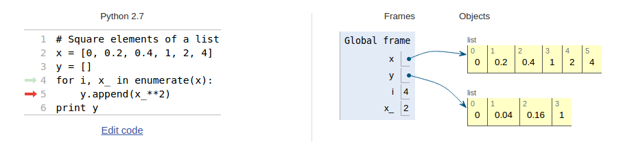
For loops

Many computations are repetitive by nature and programming languages have certain loop structures to deal with this. Here we will present what is referred to as a for loop (another kind of loop is a while loop, to be presented afterwards). Assume you want to calculate the square of each integer from 3 to 7. This could be done with the following two-line program.

for i in [3, 4, 5, 6, 7]:
    print i**2

Note the colon and indentation again!

What happens when Python interprets your code here? First of all, the word for is a reserved word signalling to Python that a for loop is wanted. Python then sticks to the rules covering such constructions and understands that, in the present example, the loop should run 5 successive times (i.e., 5 iterations should be done), letting the variable i take on the numbers \(3, 4, 5, 6, 7\) in turn. During each iteration, the statement inside the loop (i.e. print i**2) is carried out. After each iteration, i is automatically (behind the scene) updated. When the last number is reached, the last iteration is performed and the loop is finished. When executed, the program will therefore print out \(9, 16, 25, 36\) and \(49\). The variable i is often referred to as a loop index, and its name (here i) is a choice of the programmer.

Note that, had there been several statements within the loop, they would all be executed with the same value of i (before i changed in the next iteration). Make sure you understand how program execution flows here, it is important.

In Python, integer values specified for the loop variable are often produced by the built-in function range. The function range may be called in different ways, that either explicitly, or implicitly, specify the start, stop and step (i.e., change) of the loop variable. Generally, a call to range reads

range(start, stop, step)

This call makes range return the integers from (and including) start, up to (but excluding!) stop, in steps of step. Note here that stop-1 is that last integer included. With range, the previous example would rather read

for i in range(3, 8, 1):
    print i**2

By default, if range is called with only two parameters, these are taken to be start and stop, in which case a step of 1 is understood. If only a single parameter is used in the call to range, this parameter is taken to be stop. The default step of 1 is then used (combined with the starting at 0). Thus, calling range, for example, as

range(6)

would return the integers 0, 1, 2, 3, 4, 5.

Note that decreasing integers may be produced by letting start > stop combined with a negative step. This makes it easy to, e.g., traverse arrays in either direction.

Let us modify ball_plot.py from the chapter A Python program with vectorization and plotting to illustrate how useful for loops are if you need to traverse arrays. In that example we computed the height of the ball at every milli-second during the first second of its (vertical) flight and plotted the height versus time.

Assume we want to find the maximum height during that time, how can we do it with a computer program? One alternative may be to compute all the thousand heights, store them in an array, and then run through the array to pick out the maximum. The program, named ball_max_height.py, may look as follows.

import matplotlib.pyplot as plt

v0 = 5                    # Initial velocity
g = 9.81                  # Acceleration of gravity
t = linspace(0, 1, 1000)  # 1000 points in time interval
y = v0*t - 0.5*g*t**2     # Generate all heights

# At this point, the array y with all the heights is ready.
# Now we need to find the largest value within y.

largest_height = y[0]          # Starting value for search
for i in range(1, 1000):
    if y[i] > largest_height:
        largest_height = y[i]

print "The largest height achieved was %f m" % (largest_height)

# We might also like to plot the path again just to compare
plt.plot(t,y)
plt.xlabel('Time (s)')
plt.ylabel('Height (m)')
plt.show()

There is nothing new here, except the for loop construction, so let us look at it in more detail. As explained above, Python understands that a for loop is desired when it sees the word for. The range() function will produce integers from, and including, \(1\), up to, and including, \(999\), i.e. \(1000 - 1\). The value in y[0] is used as the preliminary largest height, so that, e.g., the very first check that is made is testing whether y[1] is larger than this height. If so, y[1] is stored as the largest height. The for loop then updates i to 2, and continues to check y[2], and so on. Each time we find a larger number, we store it. When finished, largest_height will contain the largest number from the array y. When you run the program, you get

The largest height achieved was 1.274210 m

which compares favorably to the plot that pops up.

To implement the traversing of arrays with loops and indices, is sometimes challenging to get right. You need to understand the start, stop and step length choices for an index, and also how the index should enter expressions inside the loop. At the same time, however, it is something that programmers do often, so it is important to develop the right skills on these matters.

Having one loop inside another, referred to as a double loop, is sometimes useful, e.g., when doing linear algebra. Say we want to find the maximum among the numbers stored in a \(4 \times 4\) matrix A. The code fragment could look like

largest_number = A[0][0]

for i in range(4):
    for j in range(4):
        if A[i][j] > largest_number:
            largest_number = A[i][j]

Here, all the j indices (0 - 3) will be covered for each value of index i. First, i stays fixed at i = 0, while j runs over all its indices. Then, i stays fixed at i = 1 while j runs over all its indices again, and so on. Sketch A on a piece of paper and follow the first few loop iterations by hand, then you will realize how the double loop construction works. Using two loops is just a special case of using multiple or nested loops, and utilizing more than two loops is just a straightforward extension of what was shown here. Note, however, that the loop index name in multiple loops must be unique to each of the nested loops. Note also that each nested loop may have as many code lines as desired, both before and after the next inner loop.

The vectorized computation of heights that we did in ball_plot.py (the chapter A Python program with vectorization and plotting) could alternatively have been done by traversing the time array (t) and, for each t element, computing the height according to the formula \(y = v_0t - \frac{1}{2}gt^2\). However, it is important to know that vectorization goes much quicker. So when speed is important, vectorization is valuable.

Use loops to compute sums

One important use of loops, is to calculate sums. As a simple example, assume some variable \(x\) given by the mathematical expression

\[x = \sum_{i=1}^{N}2\cdot i , \nonumber\]

i.e., summing up the \(N\) first even numbers. For some given \(N\), say \(N = 5\), \(x\) would typically be computed in a computer program as:

N = 5
x = 0
for i in range(1, N+1):
    x += 2*i
print x

Executing this code will print the number 30 to the screen. Note in particular how the accumulation variable x is initialized to zero. The value of x then gets updated with each iteration of the loop, and not until the loop is finished will x have the correct value. This way of building up the value is very common in programming, so make sure you understand it by simulating the code segment above by hand. It is a technique used with loops in any programming language.

While loops

Python also has another standard loop construction, the while loop, doing iterations with a loop index very much like the for loop. To illustrate what such a loop may look like, we consider another modification of ball_plot.py in the chapter A Python program with vectorization and plotting. We will now change it so that it finds the time of flight for the ball. Assume the ball is thrown with a slightly lower initial velocity, say \(4.5\hbox{ ms}^{-1}\), while everything else is kept unchanged. Since we still look at the first second of the flight, the heights at the end of the flight become negative. However, this only means that the ball has fallen below its initial starting position, i.e., the height where it left the hand, so there is no problem with that. In our array y we will then have a series of heights which towards the end of y become negative. Let us, in a program named ball_time.py find the time when heights start to get negative, i.e., when the ball crosses \(y=0\). The program could look like this

from numpy import linspace

v0 = 4.5                  # Initial velocity
g = 9.81                  # Acceleration of gravity
t = linspace(0, 1, 1000)  # 1000 points in time interval
y = v0*t - 0.5*g*t**2     # Generate all heights

# Find where the ball hits y=0
i = 0
while y[i] >= 0:
    i += 1

# Now, y[i-1]>0 and y[i]<0 so let's take the middle point
# in time as the approximation for when the ball hits h=0
print "y=0 at", 0.5*(t[i-1] + t[i])

# We plot the path again just for comparison
import matplotlib.pyplot as plt
plt.plot(t, y)
plt.plot(t, 0*t, 'g--')
plt.xlabel('Time (s)')
plt.ylabel('Height (m)')
plt.show()

If you type and run this program you should get

y=0 at 0.917417417417

The new thing here is the while loop only. The loop (note colon and indentation) will run as long as the boolean expression y[i] > 0 evaluates to True. Note that the programmer introduced a variable (the loop index) by the name i, initialized it (i = 0) before the loop, and updated it (i += 1) in the loop. So for each iteration, i is explicitly increased by 1, allowing a check of successive elements in the array y.

Compared to a for loop, the programmer does not have to specify the number of iterations when coding a while loop. It simply runs until the boolean expression becomes False. Thus, a loop index (as we have in a for loop) is not required. Furthermore, if a loop index is used in a while loop, it is not increased automatically; it must be done explicitly by the programmer. Of course, just as in for loops and if blocks, there might be (arbitrarily) many code lines in a while loop. Any for loop may also be implemented as a while loop, but while loops are more general so not all of them can be expressed as a for loop.

A problem to be aware of, is what is usually referred to as an infinite loop. In those unintentional (erroneous) cases, the boolean expression of the while test never evaluates to False, and the program can not escape the loop. This is one of the most frequent errors you will experience as a beginning programmer. If you accidentally enter an infinite loop and the program just hangs forever, press Ctrl+c to stop the program.

Lists and tuples - alternatives to arrays

We have seen that a group of numbers may be stored in an array that we may treat as a whole, or element by element. In Python, there is another way of organizing data that actually is much used, at least in non-numerical contexts, and that is a construction called list.

A list is quite similar to an array in many ways, but there are pros and cons to consider. For example, the number of elements in a list is allowed to change, whereas arrays have a fixed length that must be known at the time of memory allocation. Elements in a list can be of different type, i.e you may mix integers, floats and strings, whereas elements in an array must be of the same type. In general, lists provide more flexibility than do arrays. On the other hand, arrays give faster computations than lists, making arrays the prime choice unless the flexibility of lists is needed. Arrays also require less memory use and there is a lot of ready-made code for various mathematical operations. Vectorization requires arrays to be used.

The range() function that we used above in our for loop actually returns a list. If you for example write range(5) at the prompt in ipython, you get [0, 1, 2, 3, 4] in return, i.e., a list with 5 numbers. In a for loop, the line for i in range[5] makes i take on each of the numbers \(0, 1, 2, 3, 4\) in turn, as we saw above. Writing, e.g., x = range(5), gives a list by the name x, containing those five numbers. These numbers may now be accessed (e.g., as x[2], which contains the number 2) and used in computations just as we saw for array elements. As with arrays, indices run from \(0\) to \(n - 1\), when n is the number of elements in a list. You may convert a list to an array by x = array(L).

A list may also be created by simply writing, e.g.,

x = ['hello', 4, 3.14, 6]

giving a list where x[0] contains the string hello, x[1] contains the integer 4, etc. We may add and/or delete elements anywhere in the list as shown in the following example.

x = ['hello', 4, 3.14, 6]
x.insert(0, -2) # x then becomes [-2, 'hello', 4, 3.14, 6]
del x[3]        # x then becomes [-2, 'hello', 4, 6]
x.append(3.14)  # x then becomes [-2, 'hello', 4, 6, 3.14]

Note the ways of writing the different operations here. Using append() will always increase the list at the end. If you like, you may create an empty list as x = [] before you enter a loop which appends element by element. If you need to know the length of the list, you get the number of elements from len(x), which in our case is 5, after appending 3.14 above. This function is handy if you want to traverse all list elements by index, since range(len(x)) gives you all legal indices. Note that there are many more operations on lists possible than shown here.

Previously, we saw how a for loop may run over array elements. When we want to do the same with a list in Python, we may do it as this little example shows,

x = ['hello', 4, 3.14, 6]
for e in x:
    print 'x element: ', e
print 'This was all the elements in the list x'

This is how it usually is done in Python, and we see that e runs over the elements of x directly, avoiding the need for indexing. Be aware, however, that when loops are written like this, you can not change any element in x by “changing” e. That is, writing e += 2 will not change anything in x, since e can only be used to read (as opposed to overwrite) the list elements.

There is a special construct in Python that allows you to run through all elements of a list, do the same operation on each, and store the new elements in another list. It is referred to as list comprehension and may be demonstrated as follows.

List_1 = [1, 2, 3, 4]
List_2 = [e*10 for e in List_1]

This will produce a new list by the name List_2, containing the elements 10, 20, 30 and 40, in that order. Notice the syntax within the brackets for List_2, for e in List_1 signals that e is to successively be each of the list elements in List_1, and for each e, create the next element in List_2 by doing e*10. More generally, the syntax may be written as

List_2 = [E(e) for e in List_1]

where E(e) means some expression involving e.

In some cases, it is required to run through 2 (or more) lists at the same time. Python has a handy function called zip for this purpose. An example of how to use zip is provided in the code file_handling.py below.

We should also briefly mention about tuples, which are very much like lists, the main difference being that tuples cannot be changed. To a freshman, it may seem strange that such “constant lists” could ever be preferable over lists. However, the property of being constant is a good safeguard against unintentional changes. Also, it is quicker for Python to handle data in a tuple than in a list, which contributes to faster code. With the data from above, we may create a tuple and print the content by writing

x = ('hello', 4, 3.14, 6)
for e in x:
    print 'x element: ', e
print 'This was all the elements in the tuple x'

Trying insert or append for the tuple gives an error message (because it cannot be changed), stating that the tuple object has no such attribute.

Reading from and writing to files

Input data for a program often come from files and the results of the computations are often written to file. To illustrate basic file handling, we consider an example where we read \(x\) and \(y\) coordinates from two columns in a file, apply a function \(f\) to the \(y\) coordinates, and write the results to a new two-column data file. The first line of the input file is a heading that we can just skip:

# x and y coordinates
1.0  3.44
2.0  4.8
3.5  6.61
4.0  5.0

The relevant Python lines for reading the numbers and writing out a similar file are given in the file file_handling.py

filename = 'tmp.dat'
infile = open(filename, 'r')  # Open file for reading
line = infile.readline()      # Read first line
# Read x and y coordinates from the file and store in lists
x = []
y = []
for line in infile:
    words = line.split()      # Split line into words
    x.append(float(words[0]))
    y.append(float(words[1]))
infile.close()

# Transform y coordinates
from math import log

def f(y):
    return log(y)

for i in range(len(y)):
    y[i] = f(y[i])

# Write out x and y to a two-column file
filename = 'tmp_out.dat'
outfile = open(filename, 'w')  # Open file for writing
outfile.write('# x and y coordinates\n')
for xi, yi in zip(x, y):
    outfile.write('%10.5f %10.5f\n' % (xi, yi))
outfile.close()

Such a file with a comment line and numbers in tabular format is very common so numpy has functionality to ease reading and writing. Here is the same example using the loadtxt and savetxt functions in numpy for tabular data (file file_handling_numpy.py):

filename = 'tmp.dat'
import numpy
data = numpy.loadtxt(filename, comments='#')
x = data[:,0]
y = data[:,1]
data[:,1] = numpy.log(y)  # insert transformed y back in array
filename = 'tmp_out.dat'
filename = 'tmp_out.dat'
outfile = open(filename, 'w')  # open file for writing
outfile.write('# x and y coordinates\n')
numpy.savetxt(outfile, data, fmt='%10.5f')

Exercises

Exercise 11: Errors with colon, indent, etc.

Write the program ball_function.py as given in the text and confirm that the program runs correctly. Then save a copy of the program and use that program during the following error testing.

You are supposed to introduce errors in the code, one by one. For each error introduced, save and run the program, and comment how well Python’s response corresponds to the actual error. When you are finished with one error, re-set the program to correct behavior (and check that it works!) before moving on to the next error.

a) Change the first line from def y(t): to def y(t), i.e., remove the colon.

Solution. Running the program gives a syntax error:

    def y(t)
            ^
SyntaxError: invalid syntax

Python repeats the line where it found a problem and then tells us that the line has a syntax error. It is up to the programmer to find the error, although a little “hat” is used to show were in the line Python thinks the problem is. In this case, that “hat” is placed underneath where the colon should have been placed.

b) Remove the indent in front of the statement v0 = 5 inside the function y, i.e., shift the text four spaces to the left.

Solution. Running the program gives an indentation error:

    v0 = 5
     ^
IndentationError: expected an indented block

Python repeats the line where it suspects a missing indentation. In the error message, Python refers to a “block”, meaning that all of v0 = 5 should be shifted to the right (indented).

c) Now let the statement v0 = 5 inside the function y have an indent of three spaces (while the remaining two lines of the function have four).

Solution. Running the program gives an indentation error, differing slightly from the one we just experienced above:

    g = 9.81
    ^
IndentationError: unexpected indent

Python repeats the line where it found an unexpected indentation. The thing is that the first line (here v0 = 5) sets the minimum indentation for the function. If larger indents are to be used for succeeding lines (within the function), it must be done according to syntax rules (see the text). In the present case, indenting g = 9.81 violates the rules. Larger indents would be relevant, e.g., for the statements within a for loop.

d) Remove the left parenthesis in the first statement def y(t):

Solution. Running the program gives a syntax error:

    def yt):
          ^
SyntaxError: invalid syntax

Python repeats the line where it found the syntax problem and states that (somewhere in this line) there is a syntax error.

e) Change the first line of the function definition from def y(t): to def y():, i.e., remove the parameter t.

Solution. Running the program gives a type error:

    print y(time)

TypeError: y() takes no arguments (1 given)

Python repeats the line where it found a syntax problem and tells us that the function y is used in the wrong way, since one argument is used when calling it. To Python, this is the logical way of responding, since Python assumes our definition of the function was correct. This definition (which actually is what is wrong!) states that the function takes no parameters. By comparing with the function definition, it is up to the programmer to understand whether such an error is in the function definition (as here) or in the function call.

f) Change the first occurrence of the statement print y(time) to print y().

Solution. Running the program gives a type error:

    print y()

TypeError: y() takes exactly 1 argument (0 given)

Python repeats the line where it found a syntax problem and tells us that the function y is used in the wrong way, since no argument is used in the call. Again, Python discovered a mismatch between function definition and use of the function. Now, the definition specifies one parameter, whereas the call uses none.

Filename: errors_colon_indent_etc.py.

Exercise 12: Compare integers a and b

Explain briefly, in your own words, what the following program does.

a = input('Give an integer a: ')
b = input('Give an integer b: ')

if a < b:
    print "a is the smallest of the two numbers"
elif a == b:
    print "a and b are equal"
else:
    print "a is the largest of the two numbers"

Proceed by writing the program, and then run it a few times with different values for a and b to confirm that it works as intended. In particular, choose combinations for a and b so that all three branches of the if construction get tested.

Solution. The program takes two integers as input and checks if the number a is smaller than b, equal to b, or larger than b. A message is printed to the screen in each case.

Filename: compare_a_and_b.py.

Exercise 13: Functions for circumference and area of a circle

Write a program that takes a circle radius r as input from the user and then computes the circumference C and area A of the circle. Implement the computations of C and A as two separate functions that each takes r as input parameter. Print C and A to the screen along with an appropriate text. Run the program with \(r = 1\) and confirm that you get the right answer.

Solution. The code reads:

from math import *

def circumference(r):
    return 2*pi*r
def area(r):
    return pi*r**2

r = input('Give the radius of a circle: ')
C = circumference(r)
A = area(r)
print "Circumference: %g , Area: %g" % (C, A)

Running the program, choosing r = 1, gives the following dialog:

Give the radius of a circle: 1
Circumference: 6.28319 , Area: 3.14159

Filename: functions_circumference_area.py.

Exercise 14: Function for area of a rectangle

Write a program that computes the area \(A = b c\) of a rectangle. The values of \(b\) and \(c\) should be user input to the program. Also, write the area computation as a function that takes \(b\) and \(c\) as input parameters and returns the computed area. Let the program print the result to screen along with an appropriate text. Run the program with \(b = 2\) and \(c = 3\) to confirm correct program behavior.

Solution. The code reads:

def area(s1, s2):
    return s1*s2

b = input('Give the one side of the rectangle: ')
c = input('Give the other side of the rectangle: ')
print "Area: ", area(b, c)

Running the program, gives the following dialog:

Give the one side of the rectangle: 2
Give the other side of the rectangle: 3
Area: 6

Filename: function_area_rectangle.py.

Exercise 15: Area of a polygon

One of the most important mathematical problems through all times has been to find the area of a polygon, especially because real estate areas often had the shape of polygons, and it was necessary to pay tax for the area. We have a polygon as depicted below.

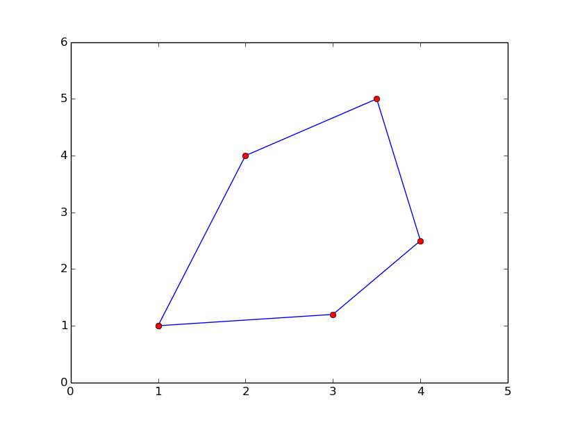
The vertices (“corners”) of the polygon have coordinates \((x_1,y_1)\), \((x_2,y_2)\), \(\ldots\), \((x_n, y_n)\), numbered either in a clockwise or counter clockwise fashion. The area \(A\) of the polygon can amazingly be computed by just knowing the boundary coordinates:

\[A = \frac{1}{2}\left| (x_1y_2+x_2y_3 + \cdots + x_{n-1}y_n + x_ny_1) - (y_1x_2 + y_2x_3 + \cdots + y_{n-1}x_n + y_nx_1)\right|\thinspace .\]

Write a function polyarea(x, y) that takes two coordinate arrays with the vertices as arguments and returns the area. Assume that x and y are either lists or arrays.

Test the function on a triangle, a quadrilateral, and a pentagon where you can calculate the area by alternative methods for comparison.

Hint. Since Python lists and arrays has 0 as their first index, it is wise to rewrite the mathematical formula in terms of vertex coordinates numbered as \(x_0,x_1,\ldots,x_{n-1}\) and \(y_0, y_1,\ldots,y_{n-1}\).

Solution. Code:

"""
Computes the area of a polygon from vertex
coordinates only.
"""

def polyarea(x, y):
    n = len(x)
    # next we may initialize area with those terms in the
    # sum that does not follow the "increasing index pattern"
    area = x[n-1]*y[0] - y[n-1]*x[0]
    for i in range(0,n-1,1):
        area += x[i]*y[i+1] - y[i]*x[i+1]
    return 0.5*abs(area)

The function can be tested, e.g., by the lines

# pentagon
x = [0, 2, 2, 1, 0]
y = [0, 0, 2, 3, 2]
print 'Area pentagon (true value = 5): ', polyarea(x, y)
# quadrilateral
x = [0, 2, 2, 0]
y = [0, 0, 2, 2]
print 'Area quadrilateral (true value = 4): ', polyarea(x, y)
# triangle
x = [0, 2, 0]
y = [0, 0, 2]
print 'Area triangle (true value = 2): ', polyarea(x, y)

which may be added after the function definition.

Filename: polyarea.py.

Exercise 16: Average of integers

Write a program that gets an integer \(N > 1\) from the user and computes the average of all integers \(i = 1,\ldots,N\). The computation should be done in a function that takes \(N\) as input parameter. Print the result to the screen with an appropriate text. Run the program with \(N = 5\) and confirm that you get the correct answer.

Solution. The code reads:

def average(N):
    sum = 0
    for i in range(1, N+1):    # Note: Must use `N+1` to get `N`
        sum += i
    return sum/float(N)

N = input('Give an integer > 1: ')
average_1_to_N = average(N)
print "The average of 1,..., %d is: %g" % (N, average_1_to_N)

Running the program, using N = 5, gives the following dialog:

Give an integer > 1: 5
The average of 1,..., 5 is: 3

Filename: average_1_to_N.py.

Exercise 17: While loop with errors

Assume some program has been written for the task of adding all integers \(i = 1,2,\ldots,10\):

some_number = 0
i = 1
while i < 11
    some_number += 1
print some_number

a) Identify the errors in the program by just reading the code and simulating the program by hand.

Solution. There is a missing colon at the end of the while loop header. Within the loop, some_number is updated by adding 1 instead of i. Finally, there is no update of the loop index i.

b) Write a new version of the program with errors corrected. Run this program and confirm that it gives the correct output.

Solution. The code reads:

some_number = 0;
i = 1
while i < 11:
    some_number += i
    i += 1
print some_number

Running the program gives 55 as the answer.

Filename: while_loop_errors.py.

Exercise 18: Area of rectangle versus circle

Consider one circle and one rectangle. The circle has a radius \(r = 10.6\). The rectangle has sides \(a\) and \(b\), but only \(a\) is known from the outset. Let \(a = 1.3\) and write a program that uses a while loop to find the largest possible integer \(b\) that gives a rectangle area smaller than, but as close as possible to, the area of the circle. Run the program and confirm that it gives the right answer (which is \(b = 271\)).

Solution. The code reads:

from math import *

r = 10.6
a = 1.3    # one side of rectangle
circle_area = pi*r**2

b = 0      # chosen starting value for other side of rectangle
while a*b < circle_area:
    b += 1
b -= 1     # must reverse the last update to get the right value
print "The largest possible value of b: ", b

Running the program gives 271 as output for b.

Filename: area_rectangle_vs_circle.py.

Exercise 19: Find crossing points of two graphs

Consider two functions \(f(x) = x\) and \(g(x) = x^2\) on the interval \([-4,4]\).

Write a program that, by trial and error, finds approximately for which values of \(x\) the two graphs cross, i.e., \(f(x) = g(x)\). Do this by considering \(N\) equally distributed points on the interval, at each point checking whether \(|f(x) - g(x)| < \epsilon\), where \(\epsilon\) is some small number. Let \(N\) and \(\epsilon\) be user input to the program and let the result be printed to screen. Run your program with \(N = 400\) and \(\epsilon = 0.01\). Explain the output from the program. Finally, try also other values of \(N\), keeping the value of \(\epsilon\) fixed. Explain your observations.

Solution. The code reads:

from numpy import *

def f(x):
    return x

def g(x):
    return x**2

N = input('Give the number of check points N: ')
epsilon = input('Give the error tolerance: ')
x_values = linspace(-4, 4, N)

# Next, we run over all indices in the array `x_values` and
# check if the difference between function values is smaller than
# the chosen limit

for i in range(N):
    if abs(f(x_values[i]) - g(x_values[i])) < epsilon:
        print x_values[i]

Running the program with 400 check-points (i.e. N = 400) and an error tolerance of 0.01 (i.e. epsilon = 0.01) gives the following dialog:

Give the number of check-points N: 400

Give the error tolerance: 0.01
0.0100250626566
0.992481203008

We note that we do not get exactly 0 and 1 (which we know are the answers). This owes to the chosen distribution of \(x\)-values. This distribution is decided by N. Trying other combinations of N and epsilon might give more than 2 “solutions”, or fewer, maybe even none. All of this boils down to whether the if test becomes true or not. For example, if you let epsilon stay constant while increasing N, you realize that the difference between \(f(x)\) and \(g(x)\) will be small for several values of \(x\), allowing more than one \(x\) value to “be a solution”. Decreasing N while epsilon is constant will eventually give no solutions, since the difference between \(f(x)\) and \(g(x)\) at the tested \(x\)-values gets too large.

Is is important here to realize the difference between the numerical test we do and the exact solution. The numerical test just gives us an approximation which we may get as “good as we want” by the right choices of N and epsilon.

Filename: crossing_2_graphs.py.

Exercise 20: Sort array with numbers

The import statement from random import * will give access to a function uniform that may be used to draw (pseudo-)random numbers from a uniform distribution between two numbers \(a\) (inclusive) and \(b\) (inclusive). For example, writing x = uniform(0,10) makes x a float value larger than, or equal to, \(0\), and smaller than, or equal to, \(10\).

Write a script that generates an array of \(6\) random numbers between \(0\) and \(10\). The program should then sort the array so that numbers appear in increasing order. Let the program make a formatted print of the array to the screen both before and after sorting. The printouts should appear on the screen so that comparison is made easy. Confirm that the array has been sorted correctly.

Solution. The code may be written as follows

from numpy import zeros
from random import uniform

N = 6
numbers = zeros(N)

# Draw random numbers
for i in range(len(numbers)):
    numbers[i] = uniform(0, 10)
print "Unsorted: %5.3f  %5.3f %5.3f %5.3f  %5.3f %5.3f" % \
        (numbers[0], numbers[1], numbers[2],\
         numbers[3], numbers[4], numbers[5])

for reference in range(N):
    smallest = numbers[reference]
    i_smallest = reference
    # Find the smallest number in remaining unprinted array
    for i in range(reference + 1, N, 1):
        if numbers[i] <= smallest:
            smallest = numbers[i]
            i_smallest = i
    # Switch numbers, and use an extra variable for that
    switch = numbers[reference]
    numbers[reference] = numbers[i_smallest]
    numbers[i_smallest] = switch

print "Sorted  : %5.3f  %5.3f %5.3f %5.3f  %5.3f %5.3f" % \
        (numbers[0], numbers[1], numbers[2],\
         numbers[3], numbers[4], numbers[5])

Filename: sort_numbers.py.

Exercise 21: Compute \(\pi\)

Up through history, great minds have developed different computational schemes for the number \(\pi\). We will here consider two such schemes, one by Leibniz (\(1646-1716\)), and one by Euler (\(1707-1783\)).

The scheme by Leibniz may be written

\[\pi = 8\sum_{k=0}^{\infty}\frac{1}{(4k + 1)(4k + 3)} , \nonumber\]

while one form of the Euler scheme may appear as

\[\pi = \sqrt[]{6\sum_{k=1}^{\infty}\frac{1}{k^2}} . \nonumber\]

If only the first \(N\) terms of each sum are used as an approximation to \(\pi\), each modified scheme will have computed \(\pi\) with some error.

Write a program that takes \(N\) as input from the user, and plots the error development with both schemes as the number of iterations approaches \(N\). Your program should also print out the final error achieved with both schemes, i.e. when the number of terms is N. Run the program with \(N = 100\) and explain briefly what the graphs show.

Solution. The code may be written as follows

from numpy import pi, zeros, sqrt

no_of_terms = input('Give number of terms in sum for pi: ')
Leibniz_error = zeros(no_of_terms)
Euler_error = zeros(no_of_terms)

#Leibniz
sum1 = 0
for k in range(0, no_of_terms):
    sum1 += 1.0/((4*k + 1)*(4*k + 3))
    Leibniz_error[k] = pi - 8*sum1
sum1 *= 8
final_Leibniz_error = abs(pi - sum1)
print "Leibniz: ", final_Leibniz_error

# Euler
sum2 = 0
for k in range(1, no_of_terms+1):  # Note index range
    sum2 += 1.0/k**2
    Euler_error[k-1] = pi - sqrt(6*sum2)
sum2 *= 6
sum2 = sqrt(sum2)
final_Euler_error = abs(pi - sum2)
print "Euler: ", final_Euler_error

import matplotlib.pyplot as plt
plt.plot(range(no_of_terms), Leibniz_error, 'b-',\
         range(no_of_terms), Euler_error, 'r-')
plt.xlabel('No of terms')
plt.ylabel('Error with Leibniz (blue) and Euler (red)')
plt.show()

Running the program as told produces the dialog

Give number of terms in sum for pi: 100
Leibniz: 0.00499996875098
Euler: 0.00951612178069

and the plot in Figure Error as a function of number of terms

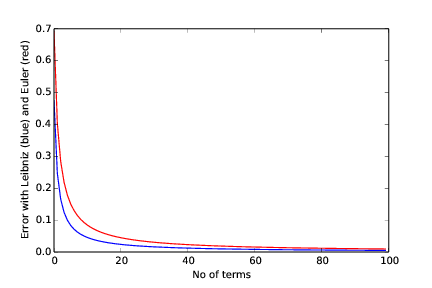
Error as a function of number of terms

We see that the scheme of Leibniz gives the least error all over the interval. However, the difference in the error with the two schemes becomes smaller as the number of terms increases.

Filename: compute_pi.py.

Exercise 22: Compute combinations of sets

Consider an ID number consisting of two letters and three digits, e.g., RE198. How many different numbers can we have, and how can a program generate all these combinations?

If a collection of \(n\) things can have \(m_1\) variations of the first thing, \(m_2\) of the second and so on, the total number of variations of the collection equals \(m_1m_2\cdots m_n\). In particular, the ID number exemplified above can have \(26\cdot 26\cdot 10\cdot 10\cdot 10 =676,000\) variations. To generate all the combinations, we must have five nested for loops. The first two run over all letters A, B, and so on to Z, while the next three run over all digits \(0,1,\ldots,9\).

To convince yourself about this result, start out with an ID number on the form A3 where the first part can vary among A, B, and C, and the digit can be among 1, 2, or 3. We must start with A and combine it with 1, 2, and 3, then continue with B, combined with 1, 2, and 3, and finally combine C with 1, 2, and 3. A double for loop does the work.

a) In a deck of cards, each card is a combination of a rank and a suit. There are 13 ranks: ace (A), 2, 3, 4, 5, 6, 7, 8, 9, 10, jack (J), queen (Q), king (K), and four suits: clubs (C), diamonds (D), hearts (H), and spades (S). A typical card may be D3. Write statements that generate a deck of cards, i.e., all the combinations CA, C2, C3, and so on to SK.

Solution. Program:

ranks = ['A', '2', '3', '4', '5', '6', '7',
         '8', '9', '10', 'J', 'Q', 'K']
suits = ['C', 'D', 'H', 'S']
deck = []
for s in suits:
    for r in ranks:
        deck.append(s + r)
print deck

b) A vehicle registration number is on the form DE562, where the letters vary from A to Z and the digits from 0 to 9. Write statements that compute all the possible registration numbers and stores them in a list.

Solution. Program:

import string
letters = string.ascii_uppercase
digits = range(10)
registration_numbers = []
for place1 in letters:
    for place2 in letters:
        for place3 in digits:
            for place4 in digits:
                for place5 in digits:
                    registration_numbers.append(
                        '%s%s%s%s%s' %
                        (place1, place2, place3, place4, place5))
print registration_numbers

c) Generate all the combinations of throwing two dice (the number of eyes can vary from 1 to 6). Count how many combinations where the sum of the eyes equals 7.

Answer. 6

Solution. Program:

dice = []
for d1 in range(1, 7):
    for d2 in range(1, 7):
        dice.append((d1, d2))

n = 0
for d1, d2 in dice:
    if d1 + d2 == 7:
        n += 1
print '%d combinations results in the sum 7' % n

Filename: combine_sets.py.

Exercise 23: Frequency of random numbers

Write a program that takes a positive integer \(N\) as input and then draws \(N\) random integers in the interval \([1,6]\) (both ends inclusive). In the program, count how many of the numbers, \(M\), that equal 6 and write out the fraction \(M/N\). Also, print all the random numbers to the screen so that you can check for yourself that the counting is correct. Run the program with a small value for N (e.g., N = 10) to confirm that it works as intended.

Hint. Use random.randint(1,6) to draw a random integer between 1 and 6.

Solution. The code may be written as follows

from random import randint

N = input('How many random numbers should be drawn? ')

# Draw random numbers
M = 0   # Counter for the occurences of 6
for i in range(N):
    drawn_number = randint(1, 6)
    print 'Draw number %d gave: %d' % (i+1, drawn_number)
    if drawn_number == 6:
        M += 1

print 'The fraction M/N became: %g' % (M/float(N))

Running the program produces the dialog

How many random numbers should be drawn? 10
Draw number 1 gave: 2
Draw number 2 gave: 4
Draw number 3 gave: 3
Draw number 4 gave: 2
Draw number 5 gave: 2
Draw number 6 gave: 1
Draw number 7 gave: 2
Draw number 8 gave: 6
Draw number 9 gave: 2
Draw number 10 gave: 3
The fraction M/N became: 0.1

We see that, in this case, 6 was drawn just a single time, so one out of ten gives a fraction M/N of \(0.1\).

Filename: count_random_numbers.py.

Remarks

For large \(N\), this program computes the probability \(M/N\) of getting six eyes when throwing a die.

Exercise 24: Game 21

Consider some game where each participant draws a series of random integers evenly distributed from \(0\) and \(10\), with the aim of getting the sum as close as possible to \(21\), but not larger than \(21\). You are out of the game if the sum passes \(21\). After each draw, you are told the number and your total sum, and is asked whether you want another draw or not. The one coming closest to \(21\) is the winner.

Implement this game in a program.

Hint. Use random.randint(0,10) to draw random integers in \([0,10]\).

Solution. The code may be written as follows

from random import randint

upper_limit = 21
not_finished = True
sum = 0
while not_finished:
    next_number = randint(0, 10)
    print "You got: ", next_number
    sum += next_number
    if sum > upper_limit:
        print "Game over, you passed 21 (with your %d points)!"\
                % sum
        not_finished = False
    else:
        print "Your score is now: %d points!" % (sum)
        answer = raw_input('Another draw (y/n)? ')
        if answer != 'y':
            not_finished = False
print "Finished!"

Running the program may produce this dialog

You got: 8
Your score is now: 8 points!

Another draw (y/n)? y
You got: 6
Your score is now: 14 points!

Another draw (y/n)? y
You got: 8
Game over, you passed 21 (with your 22 points)!

Filename: game_21.py.

Exercise 25: Linear interpolation

Some measurements \(y_i\), \(i = 1,2,\ldots,N\) (given below), of a quantity \(y\) have been collected regularly, once every minute, at times \(t_i=i\), \(i=0,1,\ldots,N\). We want to find the value \(y\) in between the measurements, e.g., at \(t=3.2\) min. Computing such \(y\) values is called interpolation.

Let your program use linear interpolation to compute \(y\) between two consecutive measurements:

1. Find \(i\) such that \(t_i\leq t \leq t_{i+1}\).
2. Find a mathematical expression for the straight line that goes through the points \((i,y_i)\) and \((i+1,y_{i+1})\).
3. Compute the \(y\) value by inserting the user’s time value in the expression for the straight line.

a) Implement the linear interpolation technique in a function that takes an array with the \(y_i\) measurements as input, together with some time \(t\), and returns the interpolated \(y\) value at time \(t\).

Solution. See the function interpolate in the script below

b) Write another function with in a loop where the user is asked for a time on the interval \([0,N]\) and the corresponding (interpolated) \(y\) value is written to the screen. The loop is terminated when the user gives a negative time.

Solution. See the function find_y in the script below

c) Use the following measurements: \(4.4, 2.0, 11.0, 21.5, 7.5\), corresponding to times \(0,1,\ldots,4\) (min), and compute interpolated values at \(t=2.5\) and \(t=3.1\) min. Perform separate hand calculations to check that the output from the program is correct.

Solution. The code may be written as follows

from numpy import zeros

def interpolate(y, t):
    """Uses linear interpolation to find intermediate y"""
    i = int(t)
    # Scheme: y(t) = y_i + delta-y/delta-t * dt
    return y[i] + ((y[i+1] - y[i])/delta_t)*(t-i)

def find_y():
    """Repeatedly finds y at t by interpolation"""
    print 'For time t on the interval [0,%d]...' % (N)
    t = input('Give your desired t > 0: ')
    while t >= 0:
        print 'y(t) = %g' % (interpolate(y, t))
        t = input('Give new time t (to stop, enter t < 0): ')

# Note: do not need to store the sequence of times
N = 4            # Total number of measurements
delta_t = 1.0    # Time difference between measurements

y = zeros(5)
y[0] = 4.4; y[1] = 2.0; y[2] = 11.0;
y[3] = 21.5; y[4] = 7.5

find_y()

Running the program may produce this dialog

For time t on the interval [0,4]...
Give your desired t: 2.5
y(t) = 16.25

Give new time t: 0.5
y(t) = 3.2

Give new time t: -1

Filename: linear_interpolation.py.

Exercise 26: Test straight line requirement

Assume the straight line function \(f(x) = 4x + 1\). Write a script that tests the “point-slope” form for this line as follows. Within a chosen interval on the \(x\)-axis (for example, for \(x\) between 0 and 10), randomly pick \(100\) points on the line and check if the following requirement is fulfilled for each point:

\[\frac{f(x_i) - f(c)}{x_i - c} = a,\hspace{.3in} i = 1,2,\ldots,100\thinspace ,\]

where \(a\) is the slope of the line and \(c\) defines a fixed point \((c,f(c))\) on the line. Let \(c = 2\) here.

Solution. The code may be written as follows

"""
For a straight line f(x) = ax + b, and the fixed point (2,f(2)) on
the line, the script tests whether (f(x_i) - f(2)) / (x_i - 2) = a
for randomly chosen x_i, i = 1,...,100.
"""

from random import random

def f(x):
    return a*x + b

a = 4.0; b = 1.0
c = 2; f_c = f(c)  # Fixed point on the line
epsilon = 1e-6
i = 0
for i in range(100):
    x = 10*random()   # random() returns number between 0 and 1
    numerator = f(x) - f_c
    denominator = x - c
    if denominator > epsilon:   # To avoid zero division
        fraction = numerator/denominator
        # The following printout should be very close to zero in
        # each case if the points are on the line
        print 'For x = %g : %g' % (x,abs(fraction - a))

The potential problem of zero division is here simply handled by the if test, meaning that if the denominator is too close to zero, that particular \(x\) is skipped. A more elegant procedure would be to use a try-except construction.

Running the program generates a printout of \(100\) lines that for each \(x\) drawn gives 0 as result from the test. The two last lines of the printout read:

For x = 2.67588 : 0
For x = 9.75893 : 0

Note that since the \(x\) values are (pseudo-)random in nature, a second run gives different values for \(x\) (but still 0 for each test!).

Filename: test_straight_line.py.

Exercise 27: Fit straight line to data

Assume some measurements \(y_i, i = 1,2,\ldots,5\) have been collected, once every second. Your task is to write a program that fits a straight line to those data.

Hint. To make your program work, you may have to insert from matplotlib.pylab import * at the top and also add show() after the plot command in the loop.

a) Make a function that computes the error between the straight line \(f(x)=ax+b\) and the measurements:

\[e = \sum_{i=1}^{5} \left(ax_i+b - y_i\right)^2\thinspace .\]

Solution. See the function find_error in the script below.

b) Make a function with a loop where you give \(a\) and \(b\), the corresponding value of \(e\) is written to the screen, and a plot of the straight line \(f(x)=ax+b\) together with the discrete measurements is shown.

Hint. To make the plotting from the loop to work, you may have to insert from matplotlib.pylab import * at the top of the script and also add show() after the plot command in the loop.

Solution. See the function interactive_line_fit in the script below.

c) Given the measurements \(0.5, 2.0, 1.0, 1.5, 7.5\), at times \(0, 1, 2, 3, 4\), use the function in b) to interactively search for \(a\) and \(b\) such that \(e\) is minimized.

Solution. The code may be written as follows

from numpy import array
import matplotlib.pyplot as plt

def f(t,a,b):
    return a*t + b

def find_error(a, b):
    E = 0
    for i in range(len(time)):
        E += (f(time[i],a,b) - data[i])**2
    return E

def interactive_line_fit():
    one_more = True
    while one_more:
        a = input('Give a: ')
        b = input('Give b: ')
        print 'The error is: %g' % (find_error(a, b))
        y = f(time, a, b)
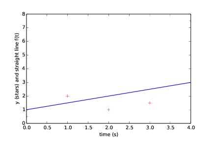
        plt.plot(time, y, time, data, '*')
        plt.xlabel('Time (s)')
        plt.ylabel('y (stars) and straight line f(t)')
        plt.show()
        answer = raw_input('Do you want another fit (y/n)? ')
        if answer == "n":
            one_more = False

data = array([0.5, 2.0, 1.0, 1.5, 7.5])
time = array([0, 1, 2, 3, 4])

interactive_line_fit()

Running the program may produce this dialog

Give a: 1
Give b: 0
The error is: 16.75

(followed by the plot seen in Figure Straight line fitted to data with first choice of line parameters (a and b))

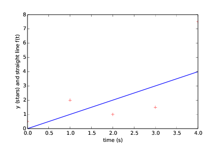
Straight line fitted to data with first choice of line parameters (a and b)

Do you want another fit (y/n)? y
Give a: 0.5
Give b: 1
The error is: 22.75

(followed by the plot seen in Figure Straight line fitted to data with second choice of line parameters (a and b))

Straight line fitted to data with second choice of line parameters (a and b)

Do you want another fit (y/n)? n

Filename: fit_straight_line.py.

Remarks

Fitting a straight line to measured data points is a very common task. The manual search procedure in c) can be automated by using a mathematical method called the method of least squares.

Exercise 28: Fit sines to straight line

A lot of technology, especially most types of digital audio devices for processing sound, is based on representing a signal of time as a sum of sine functions. Say the signal is some function \(f(t)\) on the interval \([-\pi,\pi]\) (a more general interval \([a,b]\) can easily be treated, but leads to slightly more complicated formulas). Instead of working with \(f(t)\) directly, we approximate \(f\) by the sum

\[\tag{1} S_N(t) = \sum_{n=1}^{N} b_n \sin(nt),\]

where the coefficients \(b_n\) must be adjusted such that \(S_N(t)\) is a good approximation to \(f(t)\). We shall in this exercise adjust \(b_n\) by a trial-and-error process.

a) Make a function sinesum(t, b) that returns \(S_N(t)\), given the coefficients \(b_n\) in an array b and time coordinates in an array t. Note that if t is an array, the return value is also an array.

Solution. See the script below.

b) Write a function test_sinesum() that calls sinesum(t, b) in a) and determines if the function computes a test case correctly. As test case, let t be an array with values \(-\pi/2\) and \(\pi/4\), choose \(N=2\), and \(b_1=4\) and \(b_2=-3\). Compute \(S_N(t)\) by hand to get reference values.

Solution. See the script below. Note that the call to test_sinesum is commented out, but the function will step into action if the leading # is removed.

c) Make a function plot_compare(f, N, M) that plots the original function \(f(t)\) together with the sum of sines \(S_N(t)\), so that the quality of the approximation \(S_N(t)\) can be examined visually. The argument f is a Python function implementing \(f(t)\), N is the number of terms in the sum \(S_N(t)\), and M is the number of uniformly distributed \(t\) coordinates used to plot \(f\) and \(S_N\).

Solution. See the script below.

d) Write a function error(b, f, M) that returns a mathematical measure of the error in \(S_N(t)\) as an approximation to \(f(t)\):

\[E = \sqrt{\sum_{i} \left(f(t_i) - S_N(t_i)\right)^2},\]

where the \(t_i\) values are \(M\) uniformly distributed coordinates on \([-\pi, \pi]\). The array b holds the coefficients in \(S_N\) and f is a Python function implementing the mathematical function \(f(t)\).

Solution. See the script below.

e) Make a function trial(f, N) for interactively giving \(b_n\) values and getting a plot on the screen where the resulting \(S_N(t)\) is plotted together with \(f(t)\). The error in the approximation should also be computed as indicated in d). The argument f is a Python function for \(f(t)\) and N is the number of terms \(N\) in the sum \(S_N(t)\). The trial function can run a loop where the user is asked for the \(b_n\) values in each pass of the loop and the corresponding plot is shown. You must find a way to terminate the loop when the experiments are over. Use M=500 in the calls to plot_compare and error.

Hint. To make this part of your program work, you may have to insert from matplotlib.pylab import * at the top and also add show() after the plot command in the loop.

Solution. See the script below. Note that the call to trial is commented out, but the function will run if the leading # is removed.

f) Choose \(f(t)\) to be a straight line \(f(t) = \frac{1}{\pi}t\) on \([-\pi,\pi]\). Call trial(f, 3) and try to find through experimentation some values \(b_1\), \(b_2\), and \(b_3\) such that the sum of sines \(S_N(t)\) is a good approximation to the straight line.

Solution. See the function trial in the script below.

g) Now we shall try to automate the procedure in f). Write a function that has three nested loops over values of \(b_1\), \(b_2\), and \(b_3\). Let each loop cover the interval \([-1,1]\) in steps of \(0.1\). For each combination of \(b_1\), \(b_2\), and \(b_3\), the error in the approximation \(S_N\) should be computed. Use this to find, and print, the smallest error and the corresponding values of \(b_1\), \(b_2\), and \(b_3\). Let the program also plot \(f\) and the approximation \(S_N\) corresponding to the smallest error.

Solution. The code may be written as follows

from numpy import zeros, linspace, sin, sqrt, pi, copy, arange
import matplotlib.pyplot as plt

def sinesum(t, b):
    """
    Computes S as the sum over n of b_n * sin(n*t).
    For each point in time (M) we loop over all b_n to
    produce one element S[M], i.e. one element in
    S corresponds to one point in time.
    """
    S = zeros(len(t))
    for M in range(0, len(t), 1):
        for n in range(1, len(b)+1, 1):
            S[M] += b[n-1]*sin(n*t[M])
    return S

def test_sinesum():
    t = zeros(2); t[0] = -pi/2;  t[1] = pi/4
    b = zeros(2); b[0] = 4.0;  b[1] = -3
    print sinesum(t, b)

def plot_compare(f, N, M):
    time = linspace(left_end, right_end, M)
    y = f(time)
    S = sinesum(time, b)
    plt.plot(time, y, 'b-', time, S, 'r--')
    plt.xlabel('Time')
    plt.ylabel('f (blue) and S (red)')
    plt.show()

def error(b, f, M):
    time = linspace(left_end, right_end, M)
    y = f(time)
    S = sinesum(time, b)
    E = 0
    for i in range(len(time)):
        E += sqrt((y[i] - S[i])**2)
    return E

def trial(f, N):
    M = 500
    new_trial = True
    while new_trial:
        for i in range(N):
            text = 'Give b' + str(i+1) + ' : '
            b[i] = input(text)
        plot_compare(f, N, M)
        print 'The error is: ', error(b, f, M)
        answer = raw_input('Another trial (y/n)? ')
        if answer == 'n':
            new_trial = False

def f(t):
    return (1/pi)*t

def automatic_fit(f, N):
    """Search for b-values, - just pick limits and step"""
    global b
    M = 500
    # Produce and store an initially "smallest" error
    b[0] = -1; b[1] = -1; b[2] = -1
    test_b = copy(b)
    smallest_E = error(test_b, f, M)
    db = 0.1
    for b1 in arange(-1, 1+db, db):
        for b2 in arange(-1, 1+db, db):
            for b3 in arange(-1, 1+db, db):
                test_b[0] = b1; test_b[1] = b2;
                test_b[2] = b3
                E = error(test_b, f, M)
                if E < smallest_E:
                    b = copy(test_b)
                    smallest_E = E
    plot_compare(f, N, M)
    print 'The b coeffiecients: ', b
    print 'The smallest error found: ', smallest_E

left_end = -pi;  right_end = pi
N = 3
b = zeros(N)
#test_sinesum()
#trial(f, N)
automatic_fit(f, N)

Running the program may produce this dialog

The b coefficients: [ 0.6 -0.2 0.1 ]
The smallest error found: 67.1213886326

and the plot seen in Figure Straight line fitted to data with first choice of line parameters (a and b)

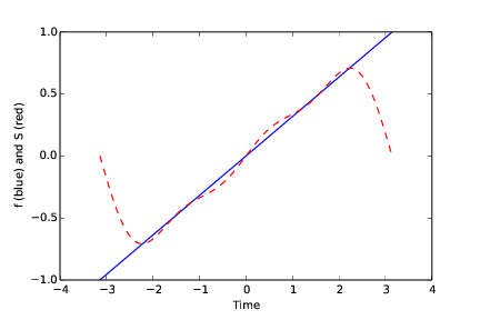
Straight line fitted to data with first choice of line parameters (a and b)

Filename: fit_sines.py.

Remarks

1. The function \(S_N(x)\) is a special case of what is called a Fourier series. At the beginning of the 19th century, Joseph Fourier (1768-1830) showed that any function can be approximated analytically by a sum of cosines and sines. The approximation improves as the number of terms (\(N\)) is increased. Fourier series are very important throughout science and engineering today.

1. Finding the coefficients \(b_n\) is solved much more accurately in Exercise 41: Revisit fit of sines to a function, by a procedure that also requires much less human and computer work!
2. In real applications, \(f(t)\) is not known as a continuous function, but function values of \(f(t)\) are provided. For example, in digital sound applications, music in a CD-quality WAV file is a signal with 44100 samples of the corresponding analog signal \(f(t)\) per second.

Exercise 29: Count occurrences of a string in a string

In the analysis of genes one encounters many problem settings involving searching for certain combinations of letters in a long string. For example, we may have a string like

gene = 'AGTCAATGGAATAGGCCAAGCGAATATTTGGGCTACCA'

We may traverse this string, letter by letter, by the for loop for letter in gene. The length of the string is given by len(gene), so an alternative traversal over an index i is for i in range(len(gene)). Letter number i is reached through gene[i], and a substring from index i up to, but not including j, is created by gene[i:j].

a) Write a function freq(letter, text) that returns the frequency of the letter letter in the string text, i.e., the number of occurrences of letter divided by the length of text. Call the function to determine the frequency of C and G in the gene string above. Compute the frequency by hand too.

b) Write a function pairs(letter, text) that counts how many times a pair of the letter letter (e.g., GG) occurs within the string text. Use the function to determine how many times the pair AA appears in the string gene above. Perform a manual counting too to check the answer.

c) Write a function mystruct(text) that counts the number of a certain structure in the string text. The structure is defined as G followed by A or T until a double GG. Perform a manual search for the structure too to control the computations by mystruct.

Solution. Here is a program:

gene = 'AGTCAATGGAATAGGCCAAGCGAATATTTGGGCTACCA'

def freq(letter, text):
    counter = 0
    for i in text:
        if i == letter:
            counter += 1
    return counter/float(len(text))

def pairs(letter, text):
    counter = 0
    for i in range(len(text)):
        if i < len(text)-1 and \
               text[i] == letter and text[i+1] == letter:
            counter += 1
    return counter

def mystruct(text):
    counter = 0
    for i in range(len(text)):
        # Search for the structure from position i
        if text[i] == 'G':
            print 'found G at', i
            # Search among A and T letters
            j = i + 1
            while text[j] == 'A' or text[j] == 'T':
                print 'next is ok:', text[j]
                j = j + 1
            print 'ending is', text[j:j+2]
            if text[j:j+2] == 'GG':
                # Correct ending of structure
                counter += 1
                print 'yes'
    return counter

print 'frequency of C: %.1f' % freq('C', gene)
print 'frequency of G: %.1f' % freq('G', gene)
print 'no of pairs AA: %d' % pairs('A', gene)
print 'no of structures: %d' % mystruct(gene)

Filename: count_substrings.py.

Remarks

You are supposed to solve the tasks using simple programming with loops and variables. While a) and b) are quite straightforward, c) quickly involves demanding logic. However, there are powerful tools available in Python that can solve the tasks efficiently in very compact code: a) text.count(letter)/float(len(text)); b) text.count(letter*2); c) len(re.findall('G[AT]+?GG', text)). That is, there is rich functionality for analysis of text in Python and this is particularly useful in analysis of gene sequences.