This chapter is taken from the book A Primer on Scientific Programming with Python by H. P. Langtangen, 5th edition, Springer, 2016.
Systems of ordinary differential equations
The software developed so far in this document targets scalar ODEs of the form \( u^{\prime}=f(u,t) \) with initial condition \( u(0)=U_0 \). Our goal now is to build flexible software for solving scalar ODEs as well as systems of ODEs. That is, we want the same code to work both for systems and scalar equations.
Mathematical problem
A scalar ODE involves the single equation $$ \begin{equation*} u^{\prime}(t) = f(u(t),t)\end{equation*} $$ with a single function \( u(t) \) as unknown, while a system of ODEs involves \( n \) scalar ODEs and consequently \( n \) unknown functions. Let us denote the unknown functions in the system by \( u^{(i)}(t) \), with \( i \) as a counter, \( i=0,\ldots,m-1 \). The system of \( n \) ODEs can then be written in the following abstract form: $$ \begin{align} {du^{(0)}\over dt} &= f^{(0)}(u^{(0)},u^{(1)},\ldots,u^{(m-1)}, t), \tag{21}\\ &\vdots&\nonumber\\ {du^{(i)}\over dt} &= f^{(i)}(u^{(0)},u^{(1)},\ldots,u^{(m-1)}, t), \tag{22}\\ &\vdots&\nonumber\\ {du^{(m-1)}\over dt} &= f^{(m-1)}(u^{(0)},u^{(1)},\ldots,u^{(m-1)}, t), \tag{23} \end{align} $$ In addition, we need \( n \) initial conditions for the \( n \) unknown functions: $$ \begin{equation} u^{(i)}(0)=U^{(i)}_0,\quad i = 0,\ldots,m-1\tp \tag{24} \end{equation} $$ Instead of writing out each equation as in (21)-(23), mathematicians like to collect the individual functions \( u^{(0)},u^{(1)},\ldots,u^{(m-1)} \) in a vector $$ \begin{equation*} u=(u^{(0)},u^{(1)},\ldots,u^{(m-1)})\tp\end{equation*} $$ The different right-hand-side functions \( f^{(0)},f^{(1)},\ldots,f^{(m-1)} \) in (21)-(23) can also be collected in a vector $$ \begin{equation*} f=(f^{(0)},f^{(1)},\ldots,f^{(m-1)})\tp\end{equation*} $$ Similarly, we put the initial conditions also in a vector $$ \begin{equation*} U_0=(U^{(0)}_0,U^{(1)}_0, \ldots,U^{(m-1)}_0)\tp\end{equation*} $$ With the vectors \( u \), \( f \), and \( U_0 \), we can write the ODE system (21)-(23) with initial conditions (24) as $$ \begin{equation} u^{\prime} = f(u, t),\quad u(0)=U_0\tp \tag{25} \end{equation} $$ This is exactly the same notation as we used for a scalar ODE (!). The power of mathematics is that abstractions can be generalized so that new problems look like the familiar ones, and very often methods carry over to the new problems in the new notation without any changes. This is true for numerical methods for ODEs too.
Let us apply the Forward Euler scheme to each of the ODEs in the system (21)-(23): $$ \begin{align} u^{(0)}_{k+1} &= u^{(0)}_{k} + \Delta t f^{(0)}(u^{(0)}_k,u^{(1)}_k,\ldots,u^{(m-1)}_k, t_k), \tag{26}\\ &\vdots&\nonumber\\ u^{(i)}_{k+1} &= u^{(i)}_{k} + \Delta t f^{(i)}(u^{(0)}_k,u^{(1)}_k,\ldots,u^{(m-1)}_k, t_k), \tag{27}\\ &\vdots&\nonumber\\ u^{(m-1)}_{k+1} &= u^{(m-1)}_{k} + \Delta t f^{(m-1)}(u^{(0)}_k,u^{(1)}_k,\ldots,u^{(m-1)}_k, t_k), \tag{28} \end{align} $$ Utilizing the vector notation, (26)-(28) can be compactly written as $$ \begin{equation} u_{k+1} = u_k + \Delta t f(u_k, t_k), \tag{29} \end{equation} $$ and this is again nothing but the formula we had for the Forward Euler scheme applied to a scalar ODE.
To summarize, the notation \( u^{\prime}=f(u,t) \), \( u(0)=U_0 \), is from now on
used both for scalar ODEs and for systems of ODEs. In the former
case, \( u \) and \( f \) are scalar functions, while in the latter case they
are vectors. This great flexibility carries over to programming too:
we can develop code for \( u^{\prime}=f(u,t) \) that works for
scalar ODEs and systems of ODEs, the only difference being that
\( u \) and \( f \) correspond to float objects for scalar ODEs and to
arrays for systems of ODEs.
Example of a system of ODEs
An oscillating spring-mass system can be governed by
a second-order
ODE:
$$
\begin{equation}
mu^{\prime\prime} + \beta u^{\prime} + ku = F(t),\quad u(0)=U_0,\ u^{\prime}(0)=0\tp \tag{30}
\end{equation}
$$
The parameters \( m \), \( \beta \), and \( k \) are known and \( F(t) \) is a
prescribed function.
This second-order equation can be rewritten as two first-order
equations by introducing two functions,
$$
\begin{equation*} u^{(0)}(t) = u(t),\quad u^{(1)}(t) = u^{\prime}(t)\tp\end{equation*}
$$
The unknowns are now the position \( u^{(0)}(t) \) and the velocity \( u^{(1)}(t) \).
We can then create equations where the derivative of the two new
primary unknowns \( u^{(0)} \) and \( u^{(1)} \) appear alone on the left-hand side:
$$
\begin{align}
{d\over dt} u^{(0)}(t) &= u^{(1)}(t),
\tag{31}\\
{d\over dt} u^{(1)}(t) &= m^{-1}(F(t) - \beta u^{(1)} - ku^{(0)})\tp
\tag{32}
\end{align}
$$
We write this system as \( u^{\prime}(t)=f(u,t) \) where
now \( u \) and \( f \) are vectors, here of length two:
$$
\begin{equation*} u(t) = (u^{(0)}(t), u^{(1)}(t))\end{equation*}
$$
$$
\begin{equation}
f(t, u) = (u^{(1)}, m^{-1}(F(t) - \beta u^{(1)} - ku^{(0)}))\tp
\tag{33}
\end{equation}
$$
Note that the vector \( u(t) \) is different from the quantity \( u \) in
(30)! There are, in fact, several interpretation of
the symbol \( u \), depending on the context: the exact solution \( u \) of
(30), the numerical solution \( u \) of
(30), the vector \( u \) in a rewrite of
(30) as a first-order ODE system, and the array u
in the software, holding the numerical approximation to \( u(t) =
(u^{(0)}(t), u^{(1)}(t)) \).
Function implementation
Let us have a look at how the software from the sections Function implementation-Switching numerical method changes if we try to
apply it to systems of ODEs.
We start with the ForwardEuler function listed
in the section Function implementation and the specific system
from the section Example of a system of ODEs.
The right-hand-side function f(u, t) must now return
the vector in (33), here as a NumPy array:
def f(u, t):
    return np.array([u[1], 1./m*(F(t) - beta*u[1] - k*u[0])])
Note that u is an array with two components, holding the
values of the two unknown functions \( u^{(0)}(t) \) and \( u^{(1)}(t) \)
at time t.
The initial conditions can also be specified as an array
U0 = np.array([0.1, 0])
What happens if we just send these f and U0 objects to the
ForwardEuler function? To answer the question, we must examine each
statement inside the function to see if the Python operations are
still valid. But of greater importance, we must check that the right
mathematics is carried out.
The first failure occurs with the statement
u = np.zeros(n+1) # u[k] is the solution at time t[k]
Now, u should be an array of arrays, since the solution at
each time level is an array. The length of U0 gives information
on how many equations and unknowns there are in the system.
An updated code is
    if isinstance(U0, (float,int)):
        u = np.zeros(n+1)
    else:
        neq = len(U0)
        u = np.zeros((n+1,neq))
Fortunately, the rest of the code now works regardless of whether
u is a one- or two-dimensional array.
In the former case, u[k+1] = u[k] + ... involves computations
with float objects only, while in the latter case,
u[k+1] picks out row \( k+1 \) in the two-dimensional array u.
This row is the
array with the two unknown values at time \( t_{k+1} \):
\( u^{(0)}(t_{k+1}) \) and \( u^{(1)}(t_{k+1}) \).
The statement u[k+1] = u[k] + ... then involves array arithmetics
with arrays of length two in this specific example.
Allowing lists
The specification of f and U0 using arrays is not as
readable as a plain list specification:
def f(u, t):
    return [u[1], 1./m*(F(t) - beta*u[1] - k*u[0])]

U0 = [0.1, 0]
Users would probably prefer the list syntax. With a little adjustment
inside the modified ForwardEuler function we can allow
lists, tuples, or arrays for U0 and as return objects from f.
With U0 we just do
U0 = np.asarray(U0)
since np.asarray will just return U0 if it already is an
array and otherwise copy the data to an array.
The situation is a bit more demanding with the f function.
The array operation
dt*f(u[k], t[k]) will not work unless f really returns an
array (since lists or tuples cannot be multiplied by a scalar dt).
A trick is to wrap a function around the user-provided
right-hand-side function:
def ForwardEuler(f_user, dt, U0, T):
    def f(u, t):
        return np.asarray(f_user(u, t))
    ...
Now, dt*f(u[k], t[k]) will call f, which calls the user's
f_user and turns whatever is returned from that function into
a NumPy array. A more compact syntax arises from using a lambda
function (see the section ref{sec:basic:lambdafunc}):
def ForwardEuler(f_user, dt, U0, T):
    f = lambda u, t: np.asarray(f_user(u, t))
    ...
The file ForwardEuler_sys_func.py contains the complete code. Verification of the implementation in terms of a test function is lacking, but Exercise 24: Code a test function for systems of ODEs encourages you to write such a function.
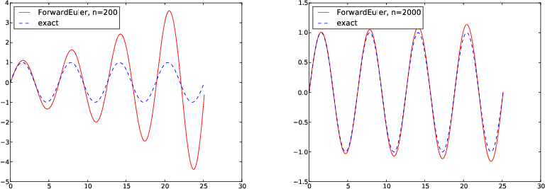
Let us apply the software to solve the equation \( u^{\prime\prime}+u=0 \), \( u(0)=0 \), \( u^{\prime}(0)=1 \), with solution \( u(t)=\sin(t) \) and \( u^{\prime}(t)=\cos(t) \). The corresponding first-order ODE system is derived in the section Example of a system of ODEs. The right-hand side of the system is in the present case \( (u^{(1)}, -u^{(0)}) \). The following Python function solves the problem
def demo(T=8*np.pi, n=200):
    def f(u, t):
        return [u[1], -u[0]]

    U0 = [0, 1]
    u, t = ForwardEuler(f, U0, T, n)
    u0 = u[:,0]

    # Plot u0 vs t and compare with exact solution sin(t)
    from matplotlib.pyplot import plot, show, savefig, legend
    plot(t, u0, 'r-', t, np.sin(t), 'b--')
    legend(['ForwardEuler, n=%d' % n, 'exact'], loc='upper left')
    savefig('tmp.pdf')
    show()
u is a
two-dimensional array where u[k,i] holds the unknown function number
\( i \) at time point number \( k \): \( u^{(i)}(t_k) \). Hence, to grab all the
values associated with \( u^{(0)} \), we fix i as 0 and let the k
index take on all its legal values: u[:,0]. This slice of the u
array refers to the piece of u where the discrete values
\( u^{(0)}(t_0),u^{(0)}(t_1), \ldots, u^{(0)}(t_{n}) \) are stored. The
remaining part of u, u[:,1], holds all the discrete values of the
computed \( u^\prime(t) \).
From visualizing the solution, see Figure 3, we realize that the Forward Euler method leads to a growing amplitude, while the exact solution has a constant amplitude. Fortunately, the amplification effect is reduced when \( \Delta t \) is reduced, but other methods, especially the 4th-order Runge-Kutta method, can solve this problem much more efficiently, see the section Example: An oscillating system.
Figure 3: Comparison of large (left) and small (right) time step when solving \( u^{\prime\prime} + u=0 \) by the Forward Euler method.
To really understand how we generalized the code for scalar ODEs to systems of ODEs, it is recommended to do Exercise 25: Code Heun's method for ODE systems; function.
Class implementation
A class version of code in the previous section naturally starts with
class ForwardEuler from the section Class implementation. The first
task is to make similar adjustments of the code as we did for the
ForwardEuler function: the trick with the lambda function for allowing
the user's f to return a list is introduced in the constructor, and
distinguishing between scalar and vector ODEs is required where
self.U0 and self.u are created. The complete class looks as
follows:
class ForwardEuler(object):
    """
    Class for solving a scalar of vector ODE,

      du/dt = f(u, t)

    by the ForwardEuler solver.

    Class attributes:
    t: array of time values
    u: array of solution values (at time points t)
    k: step number of the most recently computed solution
    f: callable object implementing f(u, t)
    """
    def __init__(self, f):
        if not callable(f):
            raise TypeError('f is %s, not a function' % type(f))
        self.f = lambda u, t: np.asarray(f(u, t))

    def set_initial_condition(self, U0):
        if isinstance(U0, (float,int)):  # scalar ODE
            self.neq = 1
        else:                            # system of ODEs
            U0 = np.asarray(U0)
            self.neq = U0.size
        self.U0 = U0

    def solve(self, time_points):
        """Compute u for t values in time_points list."""
        self.t = np.asarray(time_points)
        n = self.t.size
        if self.neq == 1:  # scalar ODEs
            self.u = np.zeros(n)
        else:              # systems of ODEs
            self.u = np.zeros((n,self.neq))

        # Assume self.t[0] corresponds to self.U0
        self.u[0] = self.U0

        # Time loop
        for k in range(n-1):
            self.k = k
            self.u[k+1] = self.advance()
        return self.u, self.t

    def advance(self):
        """Advance the solution one time step."""
        u, f, k, t = self.u, self.f, self.k, self.t
        dt = t[k+1] - t[k]
        u_new = u[k] + dt*f(u[k], t[k])
        return u_new
You are strongly encouraged to do Exercise 26: Code Heun's method for ODE systems; class
to understand class ForwardEuler listed above. This will also be
an excellent preparation for the further generalizations of class
ForwardEuler in the section The ODESolver class hierarchy.