This chapter is taken from the book A Primer on Scientific Programming with Python by H. P. Langtangen, 5th edition, Springer, 2016.

Scalar ordinary differential equations

We shall in this document work with ordinary differential equations (ODEs) written on the abstract form $$ \begin{equation} u^{\prime}(t) = f(u(t), t)\tp \tag{1} \end{equation} $$ There is an infinite number of solutions to such an equation, so to make the solution $ u(t) $ unique, we must also specify an initial condition $$ \begin{equation} u(0)=U_0\tp \tag{2} \end{equation} $$ Given $ f(u,t) $ and $ U_0 $, our task is to compute $ u(t) $.

At first sight, (1) is only a first-order differential equation, since only $ u^{\prime} $ and not higher-order derivatives like $ u^{\prime} $ are present in the equation. However, equations with higher-order derivatives can also be written on the abstract form (1) by introducing auxiliary variables and interpreting $ u $ and $ f $ as vector functions. This rewrite of the original equation leads to a system of first-order differential equations and will be treated in the section Systems of ordinary differential equations. The bottom line is that a very large family of differential equations can be written as (1). Forthcoming examples will provide evidence.

We shall first assume that $ u(t) $ is a scalar function, meaning that it has one number as value, which can be represented as a float object in Python. We then refer to (1) as a scalar differential equation. The counterpart vector function means that $ u $ is a vector of scalar functions and the equation is known as a system of ODEs (also known as a vector ODE). The value of a vector function is a list or array in a program. Systems of ODEs are treated in the section Systems of ordinary differential equations.

Examples on right-hand-side functions

To write a specific differential equation on the form (1) we need to identify what the $ f $ function is. Say the equation reads $$ \begin{equation*} y^2y' = x,\quad y(0)=Y,\end{equation*} $$ with $ y(x) $ as the unknown function. First, we need to introduce $ u $ and $ t $ as new symbols: $ u=y $, $ t=x $. This gives the equivalent equation $ u^2u^{\prime}=t $ and the initial condition $ u(0)=Y $. Second, the quantity $ u^{\prime} $ must be isolated on the left-hand side of the equation in order to bring the equation on the form (1). Dividing by $ u^2 $ gives $$ \begin{equation*} u^{\prime} = tu^{-2}\tp\end{equation*} $$ This fits the form (1), and the $ f(u,t) $ function is simply the formula involving $ u $ and $ t $ on the right-hand side: $$ \begin{equation*} f(u,t) = tu^{-2}\tp\end{equation*} $$ The $ t $ parameter is very often absent on the right-hand side such that $ f $ involves $ u $ only.

Let us list some common scalar differential equations and their corresponding $ f $ functions. Exponential growth of money or populations is governed by $$ \begin{equation} u^{\prime} = \alpha u, \tag{3} \end{equation} $$ where $ \alpha>0 $ is a given constant expressing the growth rate of $ u $. In this case, $$ \begin{equation} f(u, t) = \alpha u\tp \tag{4} \end{equation} $$ A related model is the logistic ODE for growth of a population under limited resources: $$ \begin{equation} u^{\prime} = \alpha u\left( 1-\frac{u}{R}\right), \tag{5} \end{equation} $$ where $ \alpha>0 $ is the initial growth rate and $ R $ is the maximum possible value of $ u $. The corresponding $ f $ is $$ \begin{equation} f(u, t)=\alpha u\left( 1-\frac{u}{R}\right)\tp \tag{6} \end{equation} $$ Radioactive decay of a substance has the model $$ \begin{equation} u^{\prime} = -au, \tag{7} \end{equation} $$ where $ a>0 $ is the rate of decay of $ u $. Here, $$ \begin{equation} f(u, t) = -au\tp \tag{8} \end{equation} $$ A body falling in a fluid can be modeled by $$ \begin{equation} u^{\prime} + b|u|u = g, \tag{9} \end{equation} $$ where $ b>0 $ models the fluid resistance, $ g $ is the acceleration of gravity, and $ u $ is the body's velocity (see Exercise 8: Simulate a falling or rising body in a fluid). By solving for $ u^{\prime} $ we find $$ \begin{equation} f(u,t) = -b|u|u + g\tp \tag{10} \end{equation} $$ Finally, Newton's law of cooling is the ODE $$ \begin{equation} u^{\prime} = -h(u-s), \tag{11} \end{equation} $$ where $ u $ is the temperature of a body, $ h>0 $ is a proportionality constant, normally to be estimated from experiments, and $ s $ is the temperature of the surroundings. Obviously, $$ \begin{equation} f(u, t) = -h(u-s)\tp \tag{12} \end{equation} $$

The Forward Euler scheme

Our task now is to define numerical methods for solving equations of the form (1). The simplest such method is the Forward Euler scheme. Equation (1) is to be solved for $ t\in (0,T] $, and we seek the solution $ u $ at discrete time points $ t_i=i\Delta t $, $ i=1,2,\ldots,n $. Clearly, $ t_n=n\Delta t = T $, determining the number of points $ n $ as $ T/\Delta t $. The corresponding values $ u(t_i) $ are often abbreviated as $ u_i $, just for notational simplicity.

Equation (1) is to be fulfilled at all time points $ t\in (0,T] $. However, when we solve (1) numerically, we only require the equation to be satisfied at the discrete time points $ t_1, t_2, \ldots,t_n $. That is, $$ \begin{equation*} u^{\prime}(t_k) = f(u(t_k), t_k),\end{equation*} $$ for $ k=1,\ldots,n $. The fundamental idea of the Forward Euler scheme is to approximate $ u^{\prime}(t_k) $ by a one-sided, forward difference: $$ \begin{equation*} u^{\prime}(t_k) \approx {u(t_{k+1})-u(t_k)\over \Delta t} = {u_{k+1}-u_k\over \Delta t}\tp\end{equation*} $$ This removes the derivative and leaves us with the equation $$ \begin{equation*} {u_{k+1}-u_k\over \Delta t} = f(u_k, t_k)\tp\end{equation*} $$ We assume that $ u_k $ is already computed, so that the only unknown in this equation is $ u_{k+1} $, which we can solve for: $$ \begin{equation} u_{k+1} = u_k + \Delta t f(u_k, t_k) \tp \tag{13} \end{equation} $$ This is the Forward Euler scheme for a scalar first-order differential equation $ u^{\prime}=f(u,t) $.

Equation (13) has a recursive nature. We start with the initial condition, $ u_0=U_0 $, and compute $ u_1 $ as $$ \begin{equation*} u_1 = u_0 + \Delta t f(u_0, t_0)\tp\end{equation*} $$ Then we can continue with $$ \begin{equation*} u_2 = u_1 + \Delta t f(u_1, t_1),\end{equation*} $$ and then with $ u_3 $ and so forth. This recursive nature of the method also demonstrates that we must have an initial condition – otherwise the method cannot start.

Function implementation

The next task is to write a general piece of code that implements the Forward Euler scheme (13). The complete original (continuous) mathematical problem is stated as $$ \begin{equation} u^{\prime} = f(u,t),\ t\in (0,T],\quad u(0)=U_0, \tag{14} \end{equation} $$ while the discrete numerical problem reads $$ \begin{align} u_0 & = U_0, \tag{15}\\ u_{k+1} &= u_k + \Delta t f(u_k,t_k),\ t_k=k\Delta t, k=1,\ldots, n,\ n =T/\Delta t\tp \tag{16} \end{align} $$ We see that the input data to the numerical problem consist of $ f $, $ U_0 $, $ T $, and $ \Delta t $ or $ n $. The output consists of $ u_1,u_2,\ldots,u_n $ and the corresponding set of time points $ t_1,t_2,\ldots,t_n $.

Let us implement the Forward Euler method in a function ForwardEuler that takes $ f $, $ U_0 $, $ T $, and $ n $ as input, and that returns $ u_0,\ldots,u_n $ and $ t_0,\ldots,t_n $:

import numpy as np

def ForwardEuler(f, U0, T, n):
    """Solve u'=f(u,t), u(0)=U0, with n steps until t=T."""
    t = np.zeros(n+1)
    u = np.zeros(n+1)  # u[k] is the solution at time t[k]
    u[0] = U0
    t[0] = 0
    dt = T/float(n)
    for k in range(n):
        t[k+1] = t[k] + dt
        u[k+1] = u[k] + dt*f(u[k], t[k])
    return u, t

Note the close correspondence between the implementation and the mathematical specification of the problem to be solved. The argument f to the ForwardEuler function must be a Python function f(u, t) implementing the $ f(u, t) $ function in the differential equation. In fact, f is the definition of the equation to be solved. For example, we may solve $ u^{\prime}=u $ for $ t\in (0,3) $, with $ u(0)=1 $, and $ \Delta t =0.1 $ by the following code utilizing the ForwardEuler function:

def f(u, t):
    return u

u, t = ForwardEuler(f, U0=1, T=4, n=20)

With the u and t arrays we can easily plot the solution or perform data analysis on the numbers.

Verifying the implementation

Visual comparison

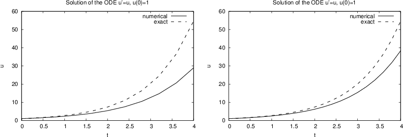
Many computational scientists and engineers look at a plot to see if a numerical and exact solution are sufficiently close, and if so, they conclude that the program works. This is, however, not a very reliable test. Consider a first try at running ForwardEuler(f, U0=1, T=4, n=10), which gives the plot to the left in Figure 1. The discrepancy between the solutions is large, and the viewer may be uncertain whether the program works correctly or not. Running n=20 should give a better solution, depicted to the right in Figure 1, but is the improvement good enough? Increasing n drives the numerical curve closer to the exact one. This brings evidence that the program is correct, but there could potentially be errors in the code that makes the curves further apart than what is implied by the numerical approximations alone. We cannot know if such a problem exists.

Figure 1: Comparison of numerical exact solution for 10 intervals (left) and 20 (intervals).

Comparing with hand calculations

A more rigorous way of verifying the implementation builds on a simple principle: we run the algorithm by hand a few times and compare the results with those in the program. For most practical purposes, it suffices to compute $ u_1 $ and $ u_2 $ by hand: $$ \begin{equation*} u_1 = 1 + 0.1\cdot 1 = 1.1,\quad u_2= 1.1 + 0.1\cdot 1.1 = 1.21\tp\end{equation*} $$ These values are to be compared with the numbers produced by the code. A correct program will lead to deviations that are zero (to machine precision). Any such test should be wrapped in a proper test function such that it can easily be repeated later. Here, it means we make a function

def test_ForwardEuler_against_hand_calculations():
    """Verify ForwardEuler against hand calc. for 3 time steps."""
    u, t = ForwardEuler(f, U0=1, T=0.2, n=2)
    exact = np.array([1, 1.1, 1.21])  # hand calculations
    error = np.abs(exact - u).max()
    success = error < 1E-14
    assert success, '|exact - u| = %g != 0' % error

The test function is written in a way that makes it trivial to integrate it in the nose testing framework. This means that the name starts with test_, there are no function arguments, and the check for passing the test is done with assert success. The test fails if the boolean variable success is False. The string after assert success is a message that will be written out if the test fails. The error measure is most conveniently a scalar number, which here is taken as the absolute value of the largest deviation between the exact and the numerical solution. Although we expect the error measure to be zero, we are prepared for rounding errors and must use a tolerance when testing if the test has passed.

Comparing with an exact numerical solution

Another effective way to verify the code, is to find a problem that can be solved exactly by the numerical method we use. That is, we seek a problem where we do not have to deal with numerical approximation errors when comparing the exact solution with the one produced by the program. It turns out that if the solution $ u(t) $ is linear in $ t $, the Forward Euler method will reproduce this solution exactly. Therefore, we choose $ u(t)=at+U_0 $, with (e.g.) $ a=0.2 $ and $ U_0=3 $. The corresponding $ f $ is the derivative of $ u $, i.e., $ f(u,t) = a $. This is obviously a very simple right-hand side without any $ u $ or $ t $. However, we can make $ f $ more complicated by adding something that is zero, e.g., some expression with $ u-(at+U_0) $, say $ (u-(at+U_0))^4 $, so that $$ \begin{equation} f(u,t) = a + (u-(at+U_0))^4\tp \tag{17} \end{equation} $$

We implement our special $ f $ and the exact solution in two functions f and u_exact, and compute a scalar measure of the error. As a above, we place the test inside a test function and make an assertion that the error is sufficiently close to zero:

def test_ForwardEuler_against_linear_solution():
    """Use knowledge of an exact numerical solution for testing."""
    def f(u, t):
        return 0.2 + (u - u_exact(t))**4

    def u_exact(t):
        return 0.2*t + 3

    u, t = ForwardEuler(f, U0=u_exact(0), T=3, n=5)
    u_e = u_exact(t)
    error = np.abs(u_e - u).max()
    success = error < 1E-14
    assert success, '|exact - u| = %g != 0' % error

A "silent" execution of the function indicates that the test works.

The shown functions are collected in a file ForwardEuler_func.py.

From discrete to continuous solution

The numerical solution of an ODE is a discrete function in the sense that we only know the function values $ u_0, u_1, ldots, u_N $ at some discrete points $ t_0, t_1, \ldots, t_N $ in time. What if we want to know $ u $ between two computed points? For example, what is $ u $ between $ t_i $ and $ t_{i+1} $, say at the midpoint $ t=t_i + \frac{1}{2}\Delta t $? One can use interpolation techniques to find this value $ u $. The simplest interpolation technique is to assume that $ u $ varies linearly on each time interval. On the interval $ [t_i, t_{i+1}] $ the linear variation of $ u $ becomes $$ \begin{equation*} u(t) = u_i + \frac{u_{i+1}-u{i}}{t_{i+1}-t_i}(t - t_i)\tp\end{equation*} $$ We can then evaluate, e.g., $ u(t_i+\frac{1}{2}\Delta t) $ from this formula and show that it becomes $ (u_i + u_{i+1})/2 $.

The function scitools.std.wrap2callable can automatically convert a discrete function to a continuous function:

from scitools.std import wrap2callable
u_cont = wrap2callable((t, u))

From the arrays t and u, wrap2callable constructs a continuous function based on linear interpolation. The result u_cont is a Python function that we can evaluate for any value of its argument t:

dt = t[i+1] - t[i]
t = t[i] + 0.5*dt
value = u_cont(t)

In general, the wrap2callable function is handy when you have computed some discrete function and you want to evaluate this discrete function at any point.

Switching numerical method

There are numerous alternative numerical methods for solving (13). One of the simplest is Heun's method: $$ \begin{align} u_* &= u_k + \Delta tf(u_k, t_k), \tag{18}\\ u_{k+1} &= u_k + \frac{1}{2}\Delta t f(u_k, t_k) + \frac{1}{2}\Delta t f(u_*, t_{k+1})\tp \tag{19} \end{align} $$ This scheme is easily implemented in the ForwardEuler function by replacing the Forward Euler formula

    u[k+1] = u[k] + dt*f(u[k], t[k])

by (18) and (19):

    u_star = u[k] + dt*f(u[k], t[k])
    u[k+1] = u[k] + 0.5*dt*f(u[k], t[k]) + 0.5*dt*f(u_star, t[k+1])

We can, especially if f is expensive to calculate, eliminate a call f(u[k], t[k]) by introducing an auxiliary variable:

    f_k = f(u[k], t[k])
    u_star = u[k] + dt*f_k
    u[k+1] = u[k] + 0.5*dt*f_k + 0.5*dt*f(u_star, t[k+1])

Class implementation

As an alternative to the general ForwardEuler function in the section Function implementation, we shall now implement the numerical method in a class. This requires, of course, familiarity with the class concept in Python.

Class wrapping of a function

Let us start with simply wrapping the ForwardEuler function in a class ForwardEuler_v1 (the postfix _v1 indicates that this is the very first class version). That is, we take the code in the ForwardEuler function and distribute it among methods in a class.

The constructor can store the input data of the problem and initialize data structures, while a solve method can perform the time stepping procedure:

import numpy as np

class ForwardEuler_v1(object):
    def __init__(self, f, U0, T, n):
        self.f, self.U0, self.T, self.n = f, dt, U0, T, n
        self.dt = T/float(n)
        self.u = np.zeros(n+1)
        self.t = np.zeros(n+1)

    def solve(self):
        """Compute solution for 0 <= t <= T."""
        self.u[0] = float(self.U0)
        self.t[0] = float(0)

        for k in range(self.n):
            self.k = k
            self.t[k+1] = self.t[k] + self.dt
            self.u[k+1] = self.advance()
        return self.u, self.t

    def advance(self):
        """Advance the solution one time step."""
        u, dt, f, k, t = \ 
           self.u, self.dt, self.f, self.k, self.t

        u_new = u[k] + dt*f(u[k], t[k])
        return u_new

Note that we have introduced a third class method, advance, which isolates the numerical scheme. The motivation is that, by observation, the constructor and the solve method are completely general as they remain unaltered if we change the numerical method (at least this is true for a wide class of numerical methods). The only difference between various numerical schemes is the updating formula. It is therefore a good programming habit to isolate the updating formula so that another scheme can be implemented by just replacing the advance method - without touching any other parts of the class.

Also note that we in the advance method "strip off" the self prefix by introducing local symbols with exactly the same names as in the mathematical specification of the numerical method. This is important if we want a visually one-to-one correspondence between the mathematics and the computer code.

Application of the class goes as follows, here for the model problem $ u^{\prime}=u $, $ u(0)=1 $:

def f(u, t):
    return u

solver = ForwardEuler_v1(f, U0=1, T=3, n=15)
u, t = solver.solve()

Switching numerical method

Implementing, for example, Heun's method (18)-(19) is a matter of replacing the advance method by

    def advance(self):
        """Advance the solution one time step."""
        u, dt, f, k, t = \ 
           self.u, self.dt, self.f, self.k, self.t

        u_star = u[k] + dt*f(u[k], t[k])
        u_new = u[k] + \ 
               0.5*dt*f(u[k], t[k]) + 0.5*dt*f(u_star, t[k+1])
        return u_new

Checking input data is always a good habit, and in the present class the constructor may test that the f argument is indeed an object that can be called as a function:

if not callable(f):
    raise TypeError('f is %s, not a function' % type(f))

Any function f or any instance of a class with a __call__ method will make callable(f) evaluate to True.

A more flexible class

Say we solve $ u^{\prime}=f(u,t) $ from $ t=0 $ to $ t=T_1 $. We can continue the solution for $ t>T_1 $ simply by restarting the whole procedure with initial conditions at $ t=T_1 $. Hence, the implementation should allow several consequtive solve steps.

Another fact is that the time step $ \Delta t $ does not need to be constant. Allowing small $ \Delta t $ in regions where $ u $ changes rapidly and letting $ \Delta t $ be larger in areas where $ u $ is slowly varying, is an attractive solution strategy. The Forward Euler method can be reformulated for a variable time step size $ t_{k+1}-t_k $: $$ \begin{equation} u_{k+1} = u_k + (t_{k+1}-t_k) f(u_k, t_k) \tp \tag{20} \end{equation} $$ Similarly, Heun's method and many other methods can be formulated with a variable step size simply by replacing $ \Delta t $ with $ t_{k+1}-t_k $. It then makes sense for the user to provide a list or array with time points for which a solution is sought: $ t_0,t_1,\ldots,t_n $. The solve method can accept such a set of points.

The mentioned extensions lead to a modified class:

class ForwardEuler(object):
    def __init__(self, f):
        if not callable(f):
            raise TypeError('f is %s, not a function' % type(f))
        self.f = f

    def set_initial_condition(self, U0):
        self.U0 = float(U0)

    def solve(self, time_points):
        """Compute u for t values in time_points list."""
        self.t = np.asarray(time_points)
        self.u = np.zeros(len(time_points))
        # Assume self.t[0] corresponds to self.U0
        self.u[0] = self.U0

        for k in range(len(self.t)-1):
            self.k = k
            self.u[k+1] = self.advance()
        return self.u, self.t

    def advance(self):
        """Advance the solution one time step."""
        u, f, k, t = self.u, self.f, self.k, self.t
        dt = t[k+1] - t[k]
        u_new = u[k] + dt*f(u[k], t[k])
        return u_new

Usage of the class

We must instantiate an instance, call the set_initial_condition method, and then call the solve method with a list or array of the time points we want to compute $ u $ at:

def f(u, t):
    """Right-hand side function for the ODE u' = u."""
    return u

solver = ForwardEuler(f)
solver.set_initial_condition(2.5)
u, t = solver.solve(np.linspace(0, 4, 21))

A simple plot(t, u) command can visualize the solution.

Verification

It is natural to perform the same verifications as we did for the ForwardEuler function in the section Verifying the implementation. First, we test the numerical solution against hand calculations. The implementation makes use of the same test function, just the way of calling up the numerical solver is different:

def test_ForwardEuler_against_hand_calculations():
    """Verify ForwardEuler against hand calc. for 2 time steps."""
    solver = ForwardEuler(lambda u, t: u)
    solver.set_initial_condition(1)
    u, t = solver.solve([0, 0.1, 0.2])
    exact = np.array([1, 1,1, 1.21])  # hand calculations
    error = np.abs(exact - u).max()
    assert error < 1E-14, '|exact - u| = %g != 0' % error

We have put some efforts into making this test very compact, mainly to demonstrate how Python allows very short, but still readable code. With a lambda function we can define the right-hand side of the ODE directly in the constructor argument. The solve method accepts a list, tuple, or array of time points and turns the data into an array anyway. Instead of a separate boolean variable success we have inserted the test inequality directly in the assert statement.

The second verification method applies the fact that the Forward Euler scheme is exact for a $ u $ that is linear in $ t $. We perform a slightly more complicated test than in the section Verifying the implementation: now we first solve for the points $ 0, 0.4, 1, 1.2 $, and then we continue the solution process for $ t_1=1.4 $ and $ t_2=1.5 $.

def test_ForwardEuler_against_linear_solution():
    """Use knowledge of an exact numerical solution for testing."""
    u_exact = lambda t: 0.2*t + 3
    solver = ForwardEuler(lambda u, t: 0.2 + (u - u_exact(t))**4)

    # Solve for first time interval [0, 1.2]
    solver.set_initial_condition(u_exact(0))
    u1, t1 = solver.solve([0, 0.4, 1, 1.2])

    # Continue with a new time interval [1.2, 1.5]
    solver.set_initial_condition(u1[-1])
    u2, t2 = solver.solve([1.2, 1.4, 1.5])

    # Append u2 to u1 and t2 to t1
    u = np.concatenate((u1, u2))
    t = np.concatenate((t1, t2))

    u_e = u_exact(t)
    error = np.abs(u_e - u).max()
    assert error < 1E-14, '|exact - u| = %g != 0' % error

Making a module

It is a well-established programming habit to have class implementations in files that act as Python modules. This means that all code is collected within classes or functions, and that the main program is executed in a test block. Upon import, no test or demonstration code should be executed.

Everything we have made so far is in classes or functions, so the remaining task to make a module, is to construct the test block.

if __name__ == '__main__':
    import sys
    if len(sys.argv) >= 2 and sys.argv[1] == 'test':
        test_ForwardEuler_v1_against_hand_calculations()
        test_ForwardEuler_against_hand_calculations()
        test_ForwardEuler_against_linear_solution()

The ForwardEuler_func.py file with functions from the sections Function implementation and Verifying the implementation is in theory a module, but not sufficiently cleaned up. Exercise 15: Clean up a file to make it a module encourages you to turn the file into a proper module.

Remark

We do not need to call the test functions from the test block, since we can let nose run the tests automatically, by nosetests -s ForwardEuler.py.

Logistic growth via a function-based approach

A more exciting application than the verification problems above is to simulate logistic growth of a population. The relevant ODE reads $$ \begin{equation*} u^{\prime}(t)=\alpha u(t)\left( 1-\frac{u(t)}{R}\right)\tp \end{equation*} $$ The mathematical $ f(u,t) $ function is simply the right-hand side of this ODE. The corresponding Python function is

def f(u, t):
    return alpha*u*(1 - u/R)

where alpha and R are global variables that correspond to $ \alpha $ and $ R $. These must be initialized before calling the ForwardEuler function (which will call the f(u,t) above):

alpha = 0.2
R = 1.0

from ForwardEuler_func2 import ForwardEuler
u, t = ForwardEuler(f, U0=0.1, T=40, n=400)

We have in this program assumed that Exercise 15: Clean up a file to make it a module has been carried out to clean up the ForwardEuler_func.py file such that it becomes a proper module file with the name ForwardEuler_func2.py.

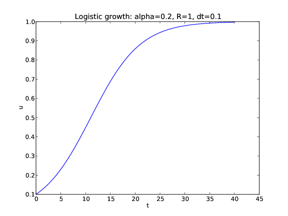
With u and t computed we can proceed with visualizing the solution (see Figure 2):

from matplotlib.pyplot import *
plot(t, u)
xlabel('t'); ylabel('u')
title('Logistic growth: alpha=%s, R=%g, dt=%g' %
      (alpha, R, t[1]-t[0]))
savefig('tmp.pdf'); savefig('tmp.png')
show()

The complete code appears in the file logistic_func.py.

Figure 2: Plot of the solution of the ODE problem $ u^{\prime} = 0.2u(1-u) $, $ u(0)=0.1 $.

Logistic growth via a class-based approach

The task of this section is to redo the implementation of the section Logistic growth via a function-based approach using a problem class to store the physical parameters and the $ f(u,t) $ function, and using class ForwardEuler from the section Class implementation to solve the ODE. Comparison with the code in the section Logistic growth via a function-based approach will then exemplify what the difference between a function-based and a class-based implementation is. There will be two major differences. One is related to technical differences between programming with functions and programming with classes. The other is psychological: when doing class programming one often puts more efforts into making more functions, a complete module, a user interface, more testing, etc. A function-based approach, and in particular the present "flat" MATLAB-style program, tends to be more ad hoc and contain less general, reusable code. At least this is the author's experience over many years when observing students and professionals create different style of code with different type of programming techniques.

The style adopted for this class-based example have several important ingredients motivated by professional programming habits:

Modules are imported as import module and calls to functions in the module are therefore prefixed with the module name such that we can easily see where different functionality comes from.
All information about the original ODE problem is collected in a class.
Physical and numerical parameters can be set on the command line.
The main program is collected in a function.
The implementation takes the form of a module such that other programs can reuse the class for representing data in a logistic problem.

The problem class

Class Logistic holds the parameters of the ODE problem: $ U_0 $, $ \alpha $, $ R $, and $ T $ as well as the $ f(u,t) $ function. Whether $ T $ should be a member of class Logistic or not is a matter of taste, but the appropriate size of $ T $ is strongly linked to the other parameters so it is natural to specify them together. The number of time intervals, $ n $, used in the numerical solution method is not a part of class Logistic since it influences the accuracy of the solution, but not the qualitative properties of the solution curve as the other parameters do.

The $ f(u,t) $ function is naturally implemented as a __call__ method such that the problem instance can act as both an instance and a callable function at the same time. In addition, we include a __str__ for printing out the ODE problem. The complete code for the class looks like

class Logistic(object):
    """Problem class for a logistic ODE."""
    def __init__(self, alpha, R, U0, T):
        self.alpha, self.R, self.U0, self.T = alpha, float(R), U0, T

    def __call__(self, u, t):
        """Return f(u,t) for the logistic ODE."""
        return self.alpha*u*(1 - u/self.R)

    def __str__(self):
        """Return ODE and initial condition."""
        return "u'(t) = %g*u*(1 - u/%g), t in [0, %g]\nu(0)=%g" % \ 
               (self.alpha, self.R, self.T, self.U0)

Getting input from the command line

We decide to specify $ \alpha $, $ R $, $ U_0 $, $ T $, and $ n $, in that order, on the command line. A function for converting the command-line arguments into proper Python objects can be

def get_input():
    """Read alpha, R, U0, T, and n from the command line."""
    try:
        alpha = float(sys.argv[1])
        R = float(sys.argv[2])
        U0 = float(sys.argv[3])
        T = float(sys.argv[4])
        n = float(sys.argv[5])
    except IndexError:
        print 'Usage: %s alpha R U0 T n' % sys.argv[0]
        sys.exit(1)
    return alpha, R, U0, T, n

We have used a standard a try-except block to handle potential errors because of missing command-line arguments. A more user-friendly alternative would be to allow option-value pairs such that, e.g., $ T $ can be set by --T 40 on the command line, but this requires more programming (with the argparse module).

Import statements

The import statements necessary for the problem solving process are written as

import ForwardEuler
import numpy as np
import matplotlib.pyplot as plt

The two latter statements with their abbreviations have evolved as a standard in Python code for scientific computing.

Solving the problem

The remaining necessary statements for solving a logistic problem are collected in a function

def logistic():
    alpha, R, U0, T, n = get_input()
    problem = Logistic(alpha=alpha, R=R, U0=U0)
    solver = ForwardEuler.ForwardEuler(problem)
    solver.set_initial_condition(problem.U0)
    time_points = np.linspace(0, T, n+1)
    u, t = solver.solve(time_points)

    plt.plot(t, u)
    plt.xlabel('t'); plt.ylabel('u')
    plt.title('Logistic growth: alpha=%s, R=%g, dt=%g'
              % (problem.alpha, problem.R, t[1]-t[0]))
    plt.savefig('tmp.pdf'); plt.savefig('tmp.png')
    plt.show()

Making a module

Everything we have created is either a class or a function. The only remaining task to ensure that the file is a proper module is to place the call to the "main" function logistic in a test block:

if __name__ == '__main__':
    logistic()

The complete module is called logistic_class.py.

Pros and cons of the class-based approach

If we quickly need to solve an ODE problem, it is tempting and efficient to go for the function-based code, because it is more direct and much shorter. A class-based module, with a user interface and often also test functions, usually gives more high-quality code that pays off when the software is expected to have a longer life time and will be extended to more complicated problems.

A pragmatic approach is to first make a quick function-based code, but refactor that code to a more reusable and extensible class version with test functions when you experience that the code frequently undergo changes. The present simple logistic ODE problem is, in my honest opinion, not complicated enough to defend a class version for practical purposes, but the primary goal here was to use a very simple mathematical problem for illustrating class programming.