This chapter is taken from the book A Primer on Scientific Programming with Python by H. P. Langtangen, 5th edition, Springer, 2016.

Exercises

Exercise 1: Implement a simple mathematical function

Implement the mathematical function $$ g(t) = e^{-t}\sin(\pi t),$$ in a Python function g(t). Print out \( g(0) \) and \( g(1) \). Filename: expsin.

Exercise 2: Implement a simple mathematical function with a parameter

Let us extend the function \( g(t) \) in Exercise 1: Implement a simple mathematical function to $$ h(t) = e^{-at}\sin(\pi t),$$ where \( a \) is a parameter. How can the corresponding Python function be implemented in this case? Print out \( h(0) \) and \( h(1) \) for the case \( a=10 \). Filename: expsin_a.

Exercise 3: Explain how a program works

Explain how the following program works:

def add(A, B):
    C = A + B
    return C

a = 3
b = 2
print add(a, b)
print add(2*a, b+1)*3

Figure out what is being printed without running the program. Filename: explain_func.

Exercise 4: Write a Fahrenheit-Celsius conversion functions

The formula for converting Fahrenheit degrees to Celsius reads $$ \begin{equation} C = \frac{5}{9}(F - 32)\tp \tag{7} \end{equation} $$ Write a function C(F) that implements this formula. Also write the inverse function F(C) for going from Celsius to Fahrenheit degrees. How can you test that the two functions work?

Hint.

Filename: f2c.

Exercise 5: Write a test function for Exercise 4: Write a Fahrenheit-Celsius conversion functions

Write a test function test_F_C that checks the computation of C(F(c)) and F(C(f)), involving the C(F) and F(C) functions in Exercise 4: Write a Fahrenheit-Celsius conversion functions.

Hint.

Filename: test_f2c.

Exercise 6: Given a test function, write the function

Here is a test function:

def test_double():
    assert double(2) == 4
    assert abs(double(0.1) - 0.2) < 1E-15
    assert double([1, 2]) == [1, 2, 1, 2]
    assert double((1, 2)) == (1, 2, 1, 2)
    assert double(3+4j) == 6+8j
    assert double('hello') == 'hellohello'

Write the associated function to be tested (double) and run test_double. Filename: test_double.

Exercise 7: Evaluate a sum and write a test function

a) Write a Python function sum_1k(M) that returns the sum \( s = \sum_{k=1}^M {1\over k} \).

b) Compute \( s \) for the case \( M=3 \) by hand and write another function test_sum_1k() that calls sum_1k(3) and checks that the answer is correct.

Hint.

Filename: sum_func.

Exercise 8: Write a function for solving \( ax^2 + bx + c =0 \)

a) Given a quadratic equation \( ax^2 + bx + c =0 \), write a function roots(a, b, c) that returns the two roots of the equation. The returned roots should be float-type objects when the roots are real, otherwise complex-type objects.

Hint.

b) Construct two test cases with known solutions, one with real roots and the other with complex roots. Implement the two test cases in two test functions test_roots_float and test_roots_complex, where you call the roots function and check the value of the returned objects.

Filename: roots_quadratic.

Exercise 9: Implement the sum function

The standard Python function called sum takes a list as argument and computes the sum of the elements in the list:

>>> sum([1,3,5,-5])
4
>>> sum([[1,2], [4,3], [8,1]])
[1, 2, 4, 3, 8, 1]
>>> sum(['Hello, ', 'World!'])
'Hello, World!'

Implement your own version of sum. Filename: mysum.

Exercise 10: Compute a polynomial via a product

Given \( n+1 \) roots \( r_0,r_1,\ldots,r_{n} \) of a polynomial \( p(x) \) of degree \( n+1 \), \( p(x) \) can be computed by $$ \begin{equation} p(x) = \prod_{i=0}^{n}(x-r_i) = (x-r_0)(x-r_1)\cdots (x-r_{n-1})(x-r_{n}) \tag{8} \tp \end{equation} $$ Write a function poly(x, roots) that takes \( x \) and a list roots of the roots as arguments and returns \( p(x) \). Construct a test case for verifying the implementation. Filename: polyprod.

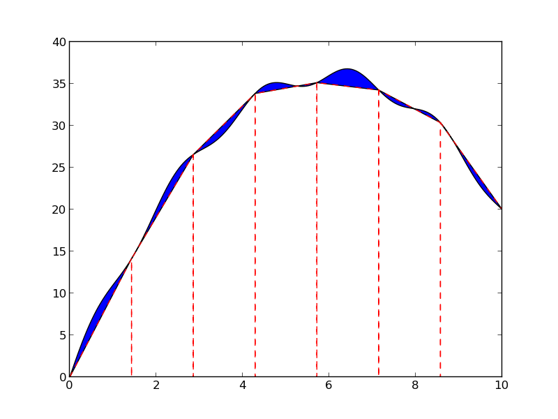
Exercise 11: Integrate a function by the Trapezoidal rule

a) An approximation to the integral of a function \( f(x) \) over an interval \( [a,b] \) can be found by first approximating \( f(x) \) by the straight line that goes through the end points \( (a,f(a)) \) and \( (b,f(b)) \), and then finding the area under the straight line, which is the area of a trapezoid. The resulting formula becomes $$ \begin{equation} \int_a^b f(x)dx \approx {b-a\over 2}(f(a) + f(b))\tp \tag{9} \end{equation} $$ Write a function trapezint1(f, a, b) that returns this approximation to the integral. The argument f is a Python implementation f(x) of the mathematical function \( f(x) \).

b) Use the approximation (9) to compute the following integrals: \( \int_0^\pi \cos x\, dx \), \( \int_0^\pi \sin x\, dx \), and \( \int_0^{\pi/2} \sin x\, dx \), In each case, write out the error, i.e., the difference between the exact integral and the approximation (9). Make rough sketches of the trapezoid for each integral in order to understand how the method behaves in the different cases.

c) We can easily improve the formula (9) by approximating the area under the function \( f(x) \) by two equal-sized trapezoids. Derive a formula for this approximation and implement it in a function trapezint2(f, a, b). Run the examples from b) and see how much better the new formula is. Make sketches of the two trapezoids in each case.

d) A further improvement of the approximate integration method from c) is to divide the area under the \( f(x) \) curve into \( n \) equal-sized trapezoids. Based on this idea, derive the following formula for approximating the integral: $$ \begin{equation} \int_a^b f(x) dx \approx \sum_{i=1}^{n-1} \frac{1}{2}h\left(f(x_{i})+f(x_{i+1}) \right), \tag{10} \end{equation} $$ where \( h \) is the width of the trapezoids, \( h = (b-a)/n \), and \( x_i=a + ih \), \( i=0,\ldots,n \), are the coordinates of the sides of the trapezoids. The figure below visualizes the idea of the Trapezoidal rule.

Implement (10) in a Python function trapezint(f, a, b, n). Run the examples from b) with \( n=10 \).

e) Write a test function test_trapezint() for verifying the implementation of the function trapezint in d).

Hint.

Filename: trapezint.

Remarks

Formula (10) is not the most common way of expressing the Trapezoidal integration rule. The reason is that \( f(x_{i+1}) \) is evaluated twice, first in term \( i \) and then as \( f(x_{i}) \) in term \( i+1 \). The formula can be further developed to avoid unnecessary evaluations of \( f(x_{i+1}) \), which results in the standard form $$ \begin{equation} \int_a^b f(x)dx\approx \frac{1}{2}h(f(a)+ f(b)) + h\sum_{i=1}^{n-1} f(x_i)\tp \tag{11} \end{equation} $$

Exercise 12: Derive the general Midpoint integration rule

The idea of the Midpoint rule for integration is to divide the area under the curve \( f(x) \) into \( n \) equal-sized rectangles (instead of trapezoids as in Exercise 11: Integrate a function by the Trapezoidal rule). The height of the rectangle is determined by the value of \( f \) at the midpoint of the rectangle. The figure below illustrates the idea.

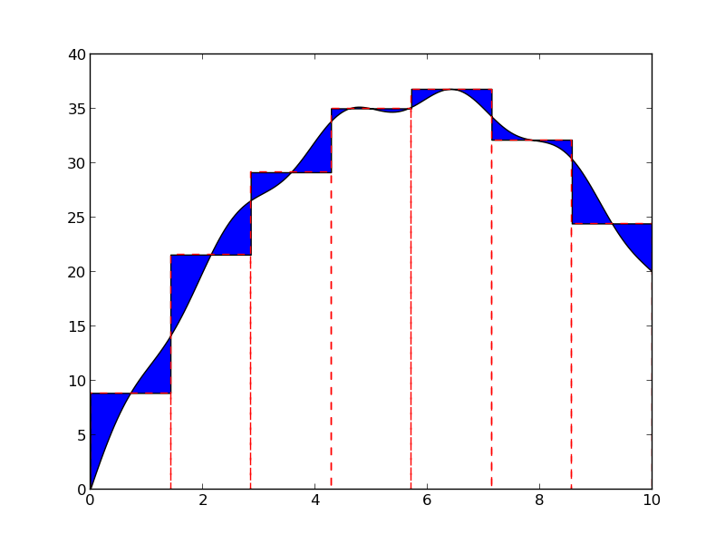
Compute the area of each rectangle, sum them up, and arrive at the formula for the Midpoint rule: $$ \begin{equation} \int_a^b f(x)dx \approx h\sum_{i=0}^{n-1} f(a + ih + \frac{1}{2}h), \tag{12} \end{equation} $$ where \( h=(b-a)/n \) is the width of each rectangle. Implement this formula in a Python function midpointint(f, a, b, n) and test the function on the examples listed in Exercise 11: Integrate a function by the Trapezoidal ruleb. How do the errors in the Midpoint rule compare with those of the Trapezoidal rule for \( n=1 \) and \( n=10 \)? Filename: midpointint.

Exercise 13: Make an adaptive Trapezoidal rule

A problem with the Trapezoidal integration rule (10) in Exercise 11: Integrate a function by the Trapezoidal rule is to decide how many trapezoids (\( n \)) to use in order to achieve a desired accuracy. Let \( E \) be the error in the Trapezoidal method, i.e., the difference between the exact integral and that produced by (10). We would like to prescribe a (small) tolerance \( \epsilon \) and find an \( n \) such that \( E\leq\epsilon \).

Since the exact value \( \int_a^bf(x)dx \) is not available (that is why we use a numerical method!), it is challenging to compute \( E \). Nevertheless, it has been shown by mathematicians that $$ \begin{equation} E \leq \frac{1}{12}(b-a)h^2\max_{x\in [a,b]}\left\vert f''(x)\right\vert\tp \tag{13} \end{equation} $$ The maximum of \( |f''(x)| \) can be computed (approximately) by evaluating \( f''(x) \) at a large number of points in \( [a,b] \), taking the absolute value \( |f''(x)| \), and finding the maximum value of these. The double derivative can be computed by a finite difference formula: $$ f''(x)\approx \frac{f(x+h) - 2f(x) + f(x-h)}{h^2}\tp$$

With the computed estimate of \( \max |f''(x)| \) we can find \( h \) from setting the right-hand side in (13) equal to the desired tolerance: $$ \begin{equation*} \frac{1}{12}(b-a)h^2\max_{x\in [a,b]}\left\vert f''(x)\right\vert = \epsilon\tp \end{equation*} $$ Solving with respect to \( h \) gives $$ \begin{equation} h = \sqrt{12\epsilon}\left( (b-a)\max_{x\in [a,b]}\left\vert f''(x)\right\vert\right)^{-1/2}\tp \tag{14} \end{equation} $$ With \( n=(b-a)/h \) we have the \( n \) that corresponds to the desired accuracy \( \epsilon \).

a) Make a Python function adaptive_trapezint(f, a, b, eps=1E-5) for computing the integral \( \int_a^b f(x)dx \) with an error less than or equal to \( \epsilon \) (eps).

Hint.

b) Apply the function to compute the integrals from Exercise 11: Integrate a function by the Trapezoidal ruleb. Write out the exact error and the estimated \( n \) for each case.

Filename: adaptive_trapezint.

Remarks

A numerical method that applies an expression for the error to adapt the choice of the discretization parameter to a desired error tolerance, is known as an adaptive numerical method. The advantage of an adaptive method is that one can control the approximation error, and there is no need for the user to determine an appropriate number of intervals \( n \).

Exercise 14: Simulate a program by hand

Simulate the following program by hand to explain what is printed.

Hint.

Filename: simulate_func.

Exercise 15: Debug a given test function

Given a Python function

def triple(x):
    return x + x*2

we want to test it with a proper test function. The following function is written

def test_triple():
    assert triple(3) == 9
    assert triple(0.1) == 0.3
    assert triple([1, 2]) == [1, 2, 1, 2, 1, 2]
    assert triple('hello ') == 'hello hello 2'

What is wrong with the test function? Write a test function where all boolean comparisons work well. Filename: test_triple.

Exercise 16: Compute the area of an arbitrary triangle

An arbitrary triangle can be described by the coordinates of its three vertices: \( (x_1,y_1) \), \( (x_2,y_2) \), \( (x_3, y_3) \), numbered in a counterclockwise direction. The area of the triangle is given by the formula $$ \begin{equation} A=\frac{1}{2}\left\vert x_2y_3 - x_3y_2 - x_1y_3 + x_3y_1 + x_1y_2 - x_2y_1\right\vert \tp \tag{15} \end{equation} $$ Write a function triangle_area(vertices) that returns the area of a triangle whose vertices are specified by the argument vertices, which is a nested list of the vertex coordinates. Make sure your implementation passes the following test function, which also illustrates how the triangle_area function works:

def test_triangle_area():
    """
    Verify the area of a triangle with vertex coordinates
    (0,0), (1,0), and (0,2).
    """
    v1 = (0,0);  v2 = (1,0);  v3 = (0,2)
    vertices = [v1, v2, v3]
    expected = 1
    computed = triangle_area(vertices)
    tol = 1E-14
    success = diff(expected - computed) < tol
    msg = 'computed area=%g != %g (expected)' % \ 
          (computed, expected)
    assert success, msg

Filename: area_triangle.

Exercise 17: Compute the length of a path

Some object is moving along a path in the plane. At \( n+1 \) points of time we have recorded the corresponding \( (x,y) \) positions of the object: \( (x_0,y_0) \), \( (x_1,y_2) \), \( \ldots \), \( (x_{n},y_{n}) \). The total length \( L \) of the path from \( (x_0,y_0) \) to \( (x_{n},y_{n}) \) is the sum of all the individual line segments (\( (x_{i-1},y_{i-1}) \) to \( (x_{i},y_{i}) \), \( i=1,\ldots,n \)): $$ \begin{equation} L = \sum_{i=1}^{n} \sqrt{ (x_i-x_{i-1})^2 + (y_i - y_{i-1})^2}\tp \tag{16} \end{equation} $$

a) Make a Python function pathlength(x, y) for computing \( L \) according to the formula. The arguments x and y hold all the \( x_0,\ldots,x_{n} \) and \( y_0,\ldots,y_{n} \) coordinates, respectively.

b) Write a test function test_pathlength() where you check that pathlength returns the correct length in a test problem.

Filename: pathlength.

Exercise 18: Approximate \( \pi \)

The value of \( \pi \) equals the circumference of a circle with radius \( 1/2 \). Suppose we approximate the circumference by a polygon through \( n+1 \) points on the circle. The length of this polygon can be found using the pathlength function from Exercise 17: Compute the length of a path. Compute \( n+1 \) points \( (x_i,y_i) \) along a circle with radius \( 1/2 \) according to the formulas $$ \begin{equation*} x_i=\frac{1}{2}\cos (2\pi i /n),\quad y_i=\frac{1}{2}\sin (2\pi i/n), \quad i=0,\ldots,n\tp \end{equation*} $$ Call the pathlength function and write out the error in the approximation of \( \pi \) for \( n=2^k \), \( k=2,3,\ldots,10 \). Filename: pi_approx.

Exercise 19: Compute the area of a polygon

One of the most important mathematical problems through all times has been to find the area of a polygon. For example, real estate areas often had the shape of polygons, and the tax was proportional to the area. Suppose we have some polygon with vertices ("corners") specified by the coordinates \( (x_1,y_1) \), \( (x_2,y_2) \), \( \ldots \), \( (x_n, y_n) \), numbered either in a clockwise or counter clockwise fashion around the polygon. The area \( A \) of the polygon can amazingly be computed by just knowing the boundary coordinates: $$ \begin{align} A = \frac{1}{2}| & (x_1y_2+x_2y_3 + \cdots + x_{n-1}y_n + x_ny_1) -\nonumber\\ & (y_1x_2 + y_2x_3 + \cdots + y_{n-1}x_n + y_nx_1)|\thinspace . \tag{17} \end{align} $$ Write a function polygon_area(x, y) that takes two coordinate lists with the vertices as arguments and returns the area.

Test the function on a triangle, a quadrilateral, and a pentagon where you can calculate the area by alternative methods for comparison.

Hint.

Filename: polygon_area.

Exercise 20: Write functions

Three functions, hw1, hw2, and hw3, work as follows:

>>> print hw1()
Hello, World!
>>> hw2()
Hello, World!
>>> print hw3('Hello, ', 'World!')
Hello, World!
>>> print hw3('Python ', 'function')
Python function

Write the three functions. Filename: hw_func.

Exercise 21: Approximate a function by a sum of sines

We consider the piecewise constant function $$ \begin{equation} \tag{18} f(t) = \left\lbrace\begin{array}{ll} 1, & 0 < t < T/2,\\ 0, & t = T/2,\\ -1, & T/2 < t < T \end{array}\right. \end{equation} $$ Sketch this function on a piece of paper. One can approximate \( f(t) \) by the sum $$ \begin{equation} S(t;n) = {4\over\pi}\sum_{i=1}^n {1\over 2i-1} \sin\left( {2(2i-1)\pi t\over T}\right)\tp \tag{19} \end{equation} $$ It can be shown that \( S(t;n)\rightarrow f(t) \) as \( n\rightarrow\infty \).

a) Write a Python function S(t, n, T) for returning the value of \( S(t;n) \).

b) Write a Python function f(t, T) for computing \( f(t) \).

c) Write out tabular information showing how the error \( f(t) - S(t;n) \) varies with \( n \) and \( t \) for the cases where \( n=1,3,5,10,30,100 \) and \( t=\alpha T \), with \( T=2\pi \), and \( \alpha =0.01, 0.25, 0.49 \). Use the table to comment on how the quality of the approximation depends on \( \alpha \) and \( n \).

Filename: sinesum1.

Remarks

A sum of sine and/or cosine functions, as in (19), is called a Fourier series. Approximating a function by a Fourier series is a very important technique in science and technology.

Exercise 22: Implement a Gaussian function

Make a Python function gauss(x, m=0, s=1) for computing the Gaussian function $$ \begin{equation*} f(x) = {1\over\sqrt{2\pi }\, s} \exp{\left[-\frac{1}{2}\left({x-m\over s}\right)^2\right]}\tp \end{equation*} $$ Write out a nicely formatted table of \( x \) and \( f(x) \) values for \( n \) uniformly spaced \( x \) values in \( [m-5s, m+5s] \). (Choose \( m \), \( s \), and \( n \) as you like.) Filename: gaussian2.

Exercise 23: Wrap a formula in a function

Implement the formula for cooking an egg, see the exercise "How to cook the perfect egg" in the document Programming with formulas, in a Python function with three arguments: egg(M, To=20, Ty=70). The parameters \( \rho \), \( K \), \( c \), and \( T_w \) can be set as local (constant) variables inside the function. Let \( t \) be returned from the function. Compute \( t \) for a soft and hard boiled egg, of a small (\( M=47 \) g) and large (\( M=67 \) g) size, taken from the fridge (\( T_o=4 \) C) and from a hot room (\( T_o=25 \) C). Filename: egg_func.

Exercise 24: Write a function for numerical differentiation

The formula $$ \begin{equation} f'(x)\approx {f(x+h)-f(x-h)\over 2h} \tag{20}\end{equation} $$ can be used to find an approximate derivative of a mathematical function \( f(x) \) if \( h \) is small.

a) Write a function diff(f, x, h=1E-5) that returns the approximation (20) of the derivative of a mathematical function represented by a Python function f(x).

b) Write a function test_diff() that verifies the implementation of the function diff. As test case, one can use the fact that (20) is exact for quadratic functions (at least for not so small \( h \) values that rounding errors in (20) become significant - you have to experiment with finding a suitable tolerance and \( h \)). Follow the conventions of the pytest and nose testing frameworks.

c) Apply (20) to differentiate

• \( f(x)=e^x \) at \( x=0 \),
• \( f(x)=e^{-2x^2} \) at \( x=0 \),
• \( f(x)=\cos x \) at \( x=2\pi \),
• \( f(x)=\ln x \) at \( x=1 \).

Filename: centered_diff.

Exercise 25: Implement the factorial function

The factorial of \( n \) is written as \( n! \) and defined as $$ \begin{equation} n! = n(n-1)(n-2)\cdots 2\cdot 1, \tag{21} \end{equation} $$ with the special cases $$ \begin{equation} 1! = 1,\quad 0! = 1\tp \tag{22} \end{equation} $$ For example, \( 4! = 4\cdot 3\cdot 2\cdot 1 = 24 \), and \( 2! = 2\cdot 1 = 2 \). Write a Python function fact(n) that returns \( n! \). (Do not simply call the ready-made function math.factorial(n) - that is considered cheating in this context!)

Make sure your fact function passes the test in the following test function:

def test_fact():
    # Check an arbitrary case
    n = 4
    expected = 4*3*2*1
    computed = fact(n)
    assert computed == expected
    # Check the special cases
    assert fact(0) == 1
    assert fact(1) == 1

Hint.

Filename: fact.

Exercise 26: Compute velocity and acceleration from 1D position data

Suppose we have recorded GPS coordinates \( x_0,\ldots,x_n \) at times \( t_0,\ldots,t_n \) while running or driving along a straight road. We want to compute the velocity \( v_i \) and acceleration \( a_i \) from these position coordinates. Using finite difference approximations, one can establish the formulas $$ \begin{align} v_i &\approx \frac{x_{i+1}-x_{i-1}}{t_{i+1}-t_{i-1}}, \tag{23}\\ a_i &\approx 2(t_{i+1}-t_{i-1})^{-1}\left(\frac{x_{i+1}-x_{i}}{t_{i+1}-t_i} - \frac{x_{i}-x_{i-1}}{t_{i}-t_{i-1}}\right), \tag{24} \end{align} $$ for \( i=1,\ldots,n-1 \) (\( v_i \) and \( a_i \) correspond to the velocity and acceleration at point \( x_i \) at time \( t_i \), respectively).

a) Write a Python function kinematics(i, x, t) for computing \( v_i \) and \( a_i \), given the arrays x and t of position and time coordinates (\( x_0,\ldots,x_n \) and \( t_0,\ldots,t_n \)).

b) Write a Python function test_kinematics() for testing the implementation in the case of constant velocity \( V \). Set \( t_0=0 \), \( t_1=0.5 \), \( t_2=1.5 \), and \( t_3=2.2 \), and \( x_i = Vt_i \). Call the kinematics function for the legal \( i \) values.

Filename: kinematics1.

Exercise 27: Find the max and min values of a function

The maximum and minimum values of a mathematical function \( f(x) \) on \( [a,b] \) can be found by computing \( f \) at a large number (\( n \)) of points and selecting the maximum and minimum values at these points. Write a Python function maxmin(f, a, b, n=1000) that returns the maximum and minimum value of a function f(x). Also write a test function for verifying the implementation for \( f(x) = \cos x \), \( x\in [-\pi/2, 2\pi] \).

Hint.

Filename: maxmin_f.

Exercise 28: Find the max and min elements in a list

Given a list a, the max function in Python's standard library computes the largest element in a: max(a). Similarly, min(a) returns the smallest element in a. Write your own max and min functions.

Hint.

Filename: maxmin_list.

Exercise 29: Implement the Heaviside function

The following step function is known as the Heaviside function and is widely used in mathematics: $$ \begin{equation} H(x) = \left\lbrace\begin{array}{ll} 0, & x < 0\\ 1, & x\geq 0 \end{array}\right. \tag{25} \end{equation} $$

a) Implement \( H(x) \) in a Python function H(x).

b) Make a Python function test_H() for testing the implementation of H(x). Compute \( H(-10) \), \( H(-10^{-15}) \), \( H(0) \), \( H(10^{-15}) \), \( H(10) \) and test that the answers are correct.

Filename: Heaviside.

Exercise 30: Implement a smoothed Heaviside function

The Heaviside function (25) listed in Exercise 29: Implement the Heaviside function is discontinuous. It is in many numerical applications advantageous to work with a smooth version of the Heaviside function where the function itself and its first derivative are continuous. One such smoothed Heaviside function is $$ \begin{equation} H_{\epsilon}(x) = \left\lbrace \begin{array}{ll} 0, & x < -\epsilon,\\ \frac{1}{2} + {x\over 2\epsilon} + {1\over 2\pi}\sin\left(\pi x\over\epsilon\right), & -\epsilon \leq x \leq \epsilon\\ 1, & x > \epsilon \end{array}\right. \tag{26} \end{equation} $$

a) Implement \( H_{\epsilon}(x) \) in a Python function H_eps(x, eps=0.01).

b) Make a Python function test_H_eps() for testing the implementation of H_eps. Check the values of some \( x < -\epsilon \), \( x=-\epsilon \), \( x=0 \), \( x=\epsilon \), and some \( x>\epsilon \).

Filename: smoothed_Heaviside.

Exercise 31: Implement an indicator function

In many applications there is need for an indicator function, which is 1 over some interval and 0 elsewhere. More precisely, we define $$ \begin{equation} I(x;L,R) = \left\lbrace\begin{array}{ll} 1, & x\in [L,R],\\ 0, & \hbox{elsewhere} \end{array}\right. \tag{27} \end{equation} $$

a) Make two Python implementations of such an indicator function, one with a direct test if \( x\in [L,R] \) and one that expresses the indicator function in terms of Heaviside functions (25): $$ \begin{equation} I(x;L,R) = H(x-L)H(R-x) \tag{28} \tp \end{equation} $$

b) Make a test function for verifying the implementation of the functions in a). Check that correct values are returned for some \( x < L \), \( x=L \), \( x=(L+R)/2 \), \( x=R \), and some \( x>R \).

Filename: indicator_func.

Exercise 32: Implement a piecewise constant function

Piecewise constant functions have a lot of important applications when modeling physical phenomena by mathematics. A piecewise constant function can be defined as $$ \begin{equation} f(x) = \left\lbrace\begin{array}{ll} v_0, & x\in [x_0, x_1),\\ v_1, & x\in [x_1, x_2),\\ \vdots &\\ v_i & x\in [x_i, x_{i+1}),\\ \vdots &\\ v_n & x\in [x_n, x_{n+1}] \end{array}\right. \tag{29} \end{equation} $$ That is, we have a union of non-overlapping intervals covering the domain \( [x_0,x_{n+1}] \), and \( f(x) \) is constant in each interval. One example is the function that is -1 on \( [0,1] \), 0 on \( [1,1.5] \), and 4 on \( [1.5,2] \), where we with the notation in (29) have \( x_0=0, x_1=1, x_2=1.5, x_3=2 \) and \( v_0=-1, v_1=0, v_3=4 \).

a) Make a Python function piecewise(x, data) for evaluating a piecewise constant mathematical function as in (29) at the point x. The data object is a list of pairs \( (v_i,x_i) \) for \( i=0,\ldots,n \). For example, data is [(0, -1), (1, 0), (1.5, 4)] in the example listed above. Since \( x_{n+1} \) is not a part of the data object, we have no means for detecting whether x is to the right of the last interval \( [x_n, x_{n+1}] \), i.e., we must assume that the user of the piecewise function sends in an \( x\leq x_{n+1} \).

b) Design suitable test cases for the function piecewise and implement them in a test function test_piecewise().

Filename: piecewise_constant1.

Exercise 33: Apply indicator functions

Implement piecewise constant functions, as defined in Exercise 32: Implement a piecewise constant function, by observing that $$ \begin{equation} f(x) = \sum_{i=0}^n v_i I(x; x_{i}, x_{i+1}), \tag{30} \end{equation} $$ where \( I(x; x_{i}, x_{i+1}) \) is the indicator function from Exercise 31: Implement an indicator function. Filename: piecewise_constant2.

Exercise 34: Test your understanding of branching

Consider the following code:

def where1(x, y):
    if x > 0:
        print 'quadrant I or IV'
    if y > 0:
        print 'quadrant I or II'

def where2(x, y):
    if x > 0:
        print 'quadrant I or IV'
    elif y > 0:
        print 'quadrant II'

for x, y in (-1, 1), (1, 1):
    where1(x,y)
    where2(x,y)

What is printed? Filename: simulate_branching.

Exercise 35: Simulate nested loops by hand

Go through the code below by hand, statement by statement, and calculate the numbers that will be printed.

n = 3
for i in range(-1, n):
    if i != 0:
        print i

for i in range(1, 13, 2*n):
    for j in range(n):
        print i, j

for i in range(1, n+1):
    for j in range(i):
        if j:
            print i, j

for i in range(1, 13, 2*n):
    for j in range(0, i, 2):
        for k in range(2, j, 1):
            b = i > j > k
            if b:
                print i, j, k

You may use a debugger, or the Online Python Tutor, see the section Understanding the program flow, to control what happens when you step through the code. Filename: simulate_nested_loops.

Exercise 36: Rewrite a mathematical function

We consider the \( L(x;n) \) sum as defined in the section Computing sums and the corresponding function L3(x, epsilon) function from the section Keyword arguments. The sum \( L(x;n) \) can be written as $$ \begin{equation*} L(x;n) = \sum_{i=1}^n c_i, \quad c_i = {1\over i}\left( {x\over 1+x}\right)^{i}\tp\end{equation*} $$

a) Derive a relation between \( c_{i} \) and \( c_{i-1} \), $$ \begin{equation*} c_{i} = ac_{i-1},\end{equation*} $$ where \( a \) is an expression involving \( i \) and \( x \).

b) The relation \( c_{i}=ac_{i-1} \) means that we can start with term as \( c_1 \), and then in each pass of the loop implementing the sum \( \sum_i c_i \) we can compute the next term \( c_i \) in the sum as

term = a*term

Write a new version of the L3 function, called L3_ci(x, epsilon), that makes use of this alternative computation of the terms in the sum.

c) Write a Python function test_L3_ci() that verifies the implementation of L3_ci by comparing with the original L3 function.

Filename: L3_recursive.

Exercise 37: Make a table for approximations of \( \cos x \)

The function \( \cos (x) \) can be approximated by the sum $$ \begin{equation} C(x;n) = \sum_{j=0}^n c_j, \tag{31} \end{equation} $$ where $$ \begin{equation*} c_j = -c_{j-1}{x^2\over 2j(2j-1)},\quad j=1,2,\ldots, n,\end{equation*} $$ and \( c_0=1 \).

a) Make a Python function for computing \( C(x;n) \).

Hint.

b) Make a function for writing out a table of the errors in the approximation \( C(x;n) \) of \( \cos (x) \) for some \( x \) and \( n \) values given as arguments to the function. Let the \( x \) values run downward in the rows and the \( n \) values to the right in the columns. For example, a table for \( x=4\pi,6\pi,8\pi,10\pi \) and \( n=5, 25, 50, 100, 200 \) can look like

     x          5         25         50        100        200
   12.5664   1.61e+04   1.87e-11   1.74e-12   1.74e-12   1.74e-12
   18.8496   1.22e+06   2.28e-02   7.12e-11   7.12e-11   7.12e-11
   25.1327   2.41e+07   6.58e+04  -4.87e-07  -4.87e-07  -4.87e-07
   31.4159   2.36e+08   6.52e+09   1.65e-04   1.65e-04   1.65e-04

Observe how the error increases with \( x \) and decreases with \( n \).

Filename: cos_sum.

Exercise 38: Use None in keyword arguments

Consider the functions L2(x, n) and L3(x, epsilon) from the sections Computing sums and Keyword arguments, whose program code is found in the file lnsum.py.

Make a more flexible function L4 where we can either specify a tolerance epsilon or a number of terms n in the sum. Moreover, we can also choose whether we want the sum to be returned or the sum and the number of terms:

value, n = L4(x, epsilon=1E-8, return_n=True)
value = L4(x, n=100)

Hint.

def L3(x, n=None, epsilon=None, return_n=False):
    if n is not None:
        ...
    if epsilon is not None:
        ...

Filename: L4.

Exercise 39: Write a sort function for a list of 4-tuples

Below is a list of the nearest stars and some of their properties. The list elements are 4-tuples containing the name of the star, the distance from the sun in light years, the apparent brightness, and the luminosity. The apparent brightness is how bright the stars look in our sky compared to the brightness of Sirius A. The luminosity, or the true brightness, is how bright the stars would look if all were at the same distance compared to the Sun. The list data are found in the file stars.txt, which looks as follows:

data = [
('Alpha Centauri A',    4.3,  0.26,      1.56),
('Alpha Centauri B',    4.3,  0.077,     0.45),
('Alpha Centauri C',    4.2,  0.00001,   0.00006),
("Barnard's Star",      6.0,  0.00004,   0.0005),
('Wolf 359',            7.7,  0.000001,  0.00002),
('BD +36 degrees 2147', 8.2,  0.0003,    0.006),
('Luyten 726-8 A',      8.4,  0.000003,  0.00006),
('Luyten 726-8 B',      8.4,  0.000002,  0.00004),
('Sirius A',            8.6,  1.00,      23.6),
('Sirius B',            8.6,  0.001,     0.003),
('Ross 154',            9.4,  0.00002,   0.0005),
]

The purpose of this exercise is to sort this list with respect to distance, apparent brightness, and luminosity. Write a program that initializes the data list as above and writes out three sorted tables: star name versus distance, star name versus apparent brightness, and star name versus luminosity.

Hint.

for item in sorted(data):
    ...

def mysort(a, b):
    if a[3] < b[3]:
        return -1
    elif a[3] > b[3]:
        return 1
    else:
        return 0

sorted(data, cmp=mysort)

sorted(data, key=lambda obj: obj[3])

Filename: sorted_stars_data.

Exercise 40: Find prime numbers

The Sieve of Eratosthenes is an algorithm for finding all prime numbers less than or equal to a number \( N \). Read about this algorithm on Wikipedia and implement it in a Python program. Filename: find_primes.

Exercise 41: Resolve a problem with a function

Consider the following interactive session:

>>> def f(x):
...     if 0 <= x <= 2:
...         return x**2
...     elif 2 < x <= 4:
...         return 4
...     elif x < 0:
...         return 0
...
>>> f(2)
4
>>> f(5)
>>> f(10)

Why do we not get any output when calling f(5) and f(10)?

Hint.

Filename: fix_branching.

Exercise 42: Determine the types of some objects

Consider the following calls to the makelist function from the section Beyond mathematical functions:

l1 = makelist(0, 100, 1)
l2 = makelist(0, 100, 1.0)
l3 = makelist(-1, 1, 0.1)
l4 = makelist(10, 20, 20)
l5 = makelist([1,2], [3,4], [5])
l6 = makelist((1,-1,1), ('myfile.dat', 'yourfile.dat'))
l7 = makelist('myfile.dat', 'yourfile.dat', 'herfile.dat')

Simulate each call by hand to determine what type of objects that become elements in the returned list and what the contents of value is after one pass in the loop.

Hint.

Filename: find_object_type.

Remarks

This exercise demonstrates that we can write a function and have in mind certain types of arguments, here typically int and float objects. However, the function can be used with other (originally unintended) arguments, such as lists and strings in the present case, leading to strange and irrelevant behavior (the problem here lies in the boolean expression value <= stop which is meaningless for some of the arguments).

Exercise 43: Find an error in a program

For the formula $$ \begin{equation*} f(x)= e^{rx}\sin(mx) + e^{sx}\sin(nx)\end{equation*} $$ we have made the program

Running this code results in

NameError: global name 'expsin' is not defined

What is the problem? Simulate the program flow by hand, use the debugger to step from line to line, or use the Online Python Tutor. Correct the program. Filename: find_error_undef.

References

1. H. P. Langtangen. Debugging in Python, \emphhttp://hplgit.github.io/primer.html/doc/pub/debug, http://hplgit.github.io/primer.html/doc/pub/debug.
2. H. P. Langtangen. Python Scripting for Computational Science, 3rd edition, Texts in Computational Science and Engineering, Springer, 2009.

• ← Prev