This chapter is taken from the book A Primer on Scientific Programming with Python by H. P. Langtangen, 5th edition, Springer, 2016.

Functions

In a computer language like Python, the term function means more than just a mathematical function. A function is a collection of statements that you can execute wherever and whenever you want in the program. You may send variables to the function to influence what is getting computed by statements in the function, and the function may return new objects back to you.

In particular, functions help avoid duplicating code snippets by putting all similar snippets in a common place. This strategy saves typing and makes it easier to change the program later. Functions are also often used to just split a long program into smaller, more manageable pieces, so the program and your own thinking about it become clearer. Python comes with lots of pre-defined functions (math.sqrt, range, and len are examples we have met so far). This section explains how you can define your own functions.

Mathematical functions as Python functions

Let us start with making a Python function that evaluates a mathematical function, more precisely the function \( F(C) \) for converting Celsius degrees \( C \) to the corresponding Fahrenheit degrees \( F \): $$ \begin{equation*} F(C) = \frac{9}{5}C+32\tp \end{equation*} $$ The corresponding Python function must take \( C \) as argument and return the value \( F(C) \). The code for this looks like

def F(C):
    return (9.0/5)*C + 32

All Python functions begin with def, followed by the function name, and then inside parentheses a comma-separated list of function arguments. Here we have only one argument C. This argument acts as a standard variable inside the function. The statements to be performed inside the function must be indented. At the end of a function it is common to return a value, that is, send a value "out of the function". This value is normally associated with the name of the function, as in the present case where the returned value is the result of the mathematical function \( F(C) \).

The def line with the function name and arguments is often referred to as the function header, while the indented statements constitute the function body.

To use a function, we must call (or invoke) it. Because the function returns a value, we need to store this value in a variable or make use of it in other ways. Here are some calls to F:

temp1 = F(15.5)
a = 10
temp2 = F(a)
print F(a+1)
sum_temp = F(10) + F(20)

The returned object from F(C) is in our case a float object. The call F(C) can therefore be placed anywhere in a code where a float object would be valid. The print statement above is one example.

As another example, say we have a list Cdegrees of Celsius degrees and we want to compute a list of the corresponding Fahrenheit degrees using the F function above in a list comprehension:

Fdegrees = [F(C) for C in Cdegrees]

Yet another example may involve a slight variation of our F(C) function, where a formatted string instead of a real number is returned:

>>> def F2(C):
...     F_value = (9.0/5)*C + 32
...     return '%.1f degrees Celsius corresponds to '\ 
...            '%.1f degrees Fahrenheit' % (C, F_value)
...
>>> s1 = F2(21)
>>> s1
'21.0 degrees Celsius corresponds to 69.8 degrees Fahrenheit'

The assignment to F_value demonstrates that we can create variables inside a function as needed.

Understanding the program flow

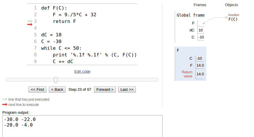
A programmer must have a deep understanding of the sequence of statements that are executed in the program and be able to simulate by hand what happens with a program in the computer. To help build this understanding, a debugger (see the document Debugging in Python [1]) or the Online Python Tutor are excellent tools. A debugger can be used for all sorts of programs, large and small, while the Online Python Tutor is primarily an educational tool for small programs. We shall demonstrate it here.

Below is a program c2f.py having a function and a for loop, with the purpose of printing out a table for conversion of Celsius to Fahrenheit degrees:

We shall now ask the Online Python Tutor to visually explain how the program is executed. Go to http://www.pythontutor.com/visualize.html, erase the code there and write or paste the c2f.py file into the editor area. Click Visualize Execution. Press the forward button to advance one statement at a time and observe the evolution of variables to the right in the window. This demo illustrates how the program jumps around in the loop and up to the F(C) function and back again. Figure 1 gives a snapshot of the status of variables, terminal output, and what the current and next statements are.

Local and global variables

Local variables are invisible outside functions

Let us reconsider the F2(C) function from the section Mathematical functions as Python functions. The variable F_value is a local variable in the function, and a local variable does not exist outside the function, i.e., in the main program. We can easily demonstrate this fact by continuing the previous interactive session:

>>> c1 = 37.5
>>> s2 = F2(c1)
>>> F_value
...
NameError: name 'F_value' is not defined

This error message demonstrates that the surrounding program outside the function is not aware of F_value. Also the argument to the function, C, is a local variable that we cannot access outside the function:

>>> C
...
NameError: name 'C' is not defined

On the contrary, the variables defined outside of the function, like s1, s2, and c1 in the above session, are global variables. These can be accessed everywhere in a program, also inside the F2 function.

Local variables hide global variables

Local variables are created inside a function and destroyed when we leave the function. To learn more about this fact, we may study the following session where we write out F_value, C, and some global variable r inside the function:

>>> def F3(C):
...     F_value = (9.0/5)*C + 32
...     print 'Inside F3: C=%s F_value=%s r=%s' % (C, F_value, r)
...     return '%.1f degrees Celsius corresponds to '\ 
...            '%.1f degrees Fahrenheit' % (C, F_value)
...
>>> C = 60    # make a global variable C
>>> r = 21    # another global variable
>>> s3 = F3(r)
Inside F3: C=21 F_value=69.8 r=21
>>> s3
'21.0 degrees Celsius corresponds to 69.8 degrees Fahrenheit'
>>> C
60

This example illustrates that there are two C variables, one global, defined in the main program with the value 60 (an int object), and one local, living when the program flow is inside the F3 function. The value of this latter C is given in the call to the F3 function (an int object). Inside the F3 function the local C hides the global C variable in the sense that when we refer to C we access the local variable. (The global C can technically be accessed as globals()['C'], but one should avoid working with local and global variables with the same names at the same time!)

The Online Python Tutor gives a complete overview of what the local and global variables are at any point of time. For instance, in the example from the section Understanding the program flow, Figure 1 shows the content of the three global variables F, dC, and C, along with the content of the variables that are in play in this call of the F(C) function: C and F.

Example

Here is a complete sample program that aims to illustrate the rule above:

print sum  # sum is a built-in Python function
sum = 500  # rebind the name sum to an int
print sum  # sum is a global variable

def myfunc(n):
    sum = n + 1
    print sum  # sum is a local variable
    return sum

sum = myfunc(2) + 1   # new value in global variable sum
print sum

In the first line, there are no local variables, so Python searches for a global value with name sum, but cannot find any, so the search proceeds with the built-in functions, and among them Python finds a function with name sum. The printout of sum becomes something like <built-in function sum>.

The second line rebinds the global name sum to an int object. When trying to access sum in the next print statement, Python searches among the global variables (no local variables so far) and finds one. The printout becomes 500. The call myfunc(2) invokes a function where sum is a local variable. Doing a print sum in this function makes Python first search among the local variables, and since sum is found there, the printout becomes 3 (and not 500, the value of the global variable sum). The value of the local variable sum is returned, added to 1, to form an int object with value 4. This int object is then bound to the global variable sum. The final print sum leads to a search among global variables, and we find one with value 4.

Changing global variables inside functions

The values of global variables can be accessed inside functions, but the values cannot be changed unless the variable is declared as global:

Note that in the f1 function, a = 21 creates a local variable a. As a programmer you may think you change the global a, but it does not happen! You are strongly encouraged to run the programs in this section in the Online Python Tutor, which is an excellent tool to explore local versus global variables and thereby get a good understanding of these concepts.

Multiple arguments

The previous F(C) and F2(C) functions from the section Mathematical functions as Python functions are functions of one variable, C, or as we phrase it in computer science: the functions take one argument (C). Functions can have as many arguments as desired; just separate the argument names by commas.

Consider the mathematical function $$ \begin{equation*} y(t) = v_0t - \frac{1}{2}gt^2,\end{equation*} $$ where \( g \) is a fixed constant and \( v_0 \) is a physical parameter that can vary. Mathematically, \( y \) is a function of one variable, \( t \), but the function values also depends on the value of \( v_0 \). That is, to evaluate \( y \), we need values for \( t \) and \( v_0 \). A natural Python implementation is therefore a function with two arguments:

def yfunc(t, v0):
    g = 9.81
    return v0*t - 0.5*g*t**2

Note that the arguments t and v0 are local variables in this function. Examples on valid calls are

y = yfunc(0.1, 6)
y = yfunc(0.1, v0=6)
y = yfunc(t=0.1, v0=6)
y = yfunc(v0=6, t=0.1)

The possibility to write argument=value in the call makes it easier to read and understand the call statement. With the argument=value syntax for all arguments, the sequence of the arguments does not matter in the call, which here means that we may put v0 before t. When omitting the argument= part, the sequence of arguments in the call must perfectly match the sequence of arguments in the function definition. The argument=value arguments must appear after all the arguments where only value is provided (e.g., yfunc(t=0.1, 6) is illegal).

Whether we write yfunc(0.1, 6) or yfunc(v0=6, t=0.1), the arguments are initialized as local variables in the function in the same way as when we assign values to variables:

    t = 0.1
    v0 = 6

These statements are not visible in the code, but a call to a function automatically initializes the arguments in this way.

Function argument or global variable?

Since \( y \) mathematically is considered a function of one variable, \( t \), some may argue that the Python version of the function, yfunc, should be a function of t only. This is easy to reflect in Python:

def yfunc(t):
    g = 9.81
    return v0*t - 0.5*g*t**2

The main difference is that v0 now becomes a global variable, which needs to be initialized outside the function yfunc (in the main program) before we attempt to call yfunc. The next session demonstrates what happens if we fail to initialize such a global variable:

>>> def yfunc(t):
...     g = 9.81
...     return v0*t - 0.5*g*t**2
...
>>> yfunc(0.6)
...
NameError: global name 'v0' is not defined

The remedy is to define v0 as a global variable prior to calling yfunc:

>>> v0 = 5
>>> yfunc(0.6)
1.2342

The rationale for having yfunc as a function of t only becomes evident in the section Functions as arguments to functions.

Beyond mathematical functions

So far our Python functions have typically computed some mathematical function, but the usefulness of Python functions goes far beyond mathematical functions. Any set of statements that we want to repeatedly execute under potentially slightly different circumstances is a candidate for a Python function. Say we want to make a list of numbers starting from some value and stopping at another value, with increments of a given size. With corresponding variables start=2, stop=8, and inc=2, we should produce the numbers 2, 4, 6, and 8. Let us write a function doing the task, together with a couple of statements that demonstrate how we call the function:

def makelist(start, stop, inc):
    value = start
    result = []
    while value <= stop:
        result.append(value)
        value = value + inc
    return result

mylist = makelist(0, 100, 0.2)
print mylist  # will print 0, 0.2, 0.4, 0.6, ... 99.8, 100

Remark 1

The makelist function has three arguments: start, stop, and inc, which become local variables in the function. Also value and result are local variables. In the surrounding program we define only one variable, mylist, and this is then a global variable.

Remark 2

You may think that range(start, stop, inc) makes the makelist function redundant, but range can only generate integers, while makelist can generate real numbers too, and more, as demonstrated in Exercise 42: Determine the types of some objects.

Multiple return values

Python functions may return more than one value. Suppose we are interested in evaluating both \( y(t) \) and \( y'(t) \): $$ \begin{align*} y(t) & = v_0t - \frac{1}{2}gt^2,\\ y'(t) & = v_0 - gt\tp \end{align*} $$ To return both \( y \) and \( y' \) we simply separate their corresponding variables by a comma in the return statement:

def yfunc(t, v0):
    g = 9.81
    y = v0*t - 0.5*g*t**2
    dydt = v0 - g*t
    return y, dydt

Calling this latter yfunc function makes a need for two values on the left-hand side of the assignment operator because the function returns two values:

position, velocity = yfunc(0.6, 3)

Here is an application of the yfunc function for producing a nicely formatted table of \( t \), \( y(t) \), and \( y'(t) \) values:

t_values = [0.05*i for i in range(10)]
for t in t_values:
    position, velocity = yfunc(t, v0=5)
    print 't=%-10g position=%-10g velocity=%-10g' % \ 
         (t, position, velocity)

The format %-10g prints a real number as compactly as possible (decimal or scientific notation) in a field of width 10 characters. The minus sign (-) after the percentage sign implies that the number is left-adjusted in this field, a feature that is important for creating nice-looking columns in the output:

t=0          position=0          velocity=5
t=0.05       position=0.237737   velocity=4.5095
t=0.1        position=0.45095    velocity=4.019
t=0.15       position=0.639638   velocity=3.5285
t=0.2        position=0.8038     velocity=3.038
t=0.25       position=0.943437   velocity=2.5475
t=0.3        position=1.05855    velocity=2.057
t=0.35       position=1.14914    velocity=1.5665
t=0.4        position=1.2152     velocity=1.076
t=0.45       position=1.25674    velocity=0.5855

When a function returns multiple values, separated by a comma in the return statement, a tuple is actually returned. We can demonstrate that fact by the following session:

>>> def f(x):
...     return x, x**2, x**4
...
>>> s = f(2)
>>> s
(2, 4, 16)
>>> type(s)
<type 'tuple'>
>>> x, x2, x4 = f(2)   # store in separate variables

Computing sums

Our next example concerns a Python function for calculating the sum $$ \begin{equation} L(x;n) = \sum_{i=1}^n {1\over i}\left( {x\over 1+x}\right)^{i}\tp \tag{1} \end{equation} $$ To compute a sum in a program, we use a loop and add terms to an accumulation variable inside the loop. For example, the implementation of \( \sum_{i=1}^n i^2 \) is typically implemented as

s = 0
for i in range(1, n+1):
    s += i**2

For the specific sum (1) we just replace i**2 by the right term inside the for loop:

s = 0
for i in range(1, n+1):
    s += (1.0/i)*(x/(1.0+x))**i

Observe the factors 1.0 used to avoid integer division, since i is int and x may also be int.

It is natural to embed the computation of the sum in a function that takes \( x \) and \( n \) as arguments and returns the sum:

def L(x, n):
    s = 0
    for i in range(1, n+1):
        s += (1.0/i)*(x/(1.0+x))**i
    return s

Our formula (1) is not chosen at random. In fact, it can be shown that \( L(x;n) \) is an approximation to \( \ln (1+x) \) for a finite \( n \) and \( x\geq 1 \). The approximation becomes exact in the limit $$ \begin{equation*} \lim_{n\rightarrow\infty} L(x;n) = \ln (1+x)\tp \end{equation*} $$

Instead of having our L function just returning the value of the sum, we could return additional information on the error involved in the approximation of \( \ln (1+x) \) by \( L(x;n) \). The size of the terms decreases with increasing \( n \), and the first neglected term is then bigger than all the remaining terms, but not necessarily bigger than their sum. The first neglected term is hence an indication of the size of the total error we make, so we may use this term as a rough estimate of the error. For comparison, we could also return the exact error since we are able to calculate the \( \ln \) function by math.log.

A new version of the L(x, n) function, where we return the value of \( L(x;n) \), the first neglected term, and the exact error goes as follows:

def L2(x, n):
    s = 0
    for i in range(1, n+1):
        s += (1.0/i)*(x/(1.0+x))**i
    value_of_sum = s
    first_neglected_term = (1.0/(n+1))*(x/(1.0+x))**(n+1)
    from math import log
    exact_error = log(1+x) - value_of_sum
    return value_of_sum, first_neglected_term, exact_error

# typical call:
value, approximate_error, exact_error = L2(x, 100)

The next section demonstrates the usage of the L2 function to judge the quality of the approximation \( L(x;n) \) to \( \ln (1+x) \).

Functions with no return values

Sometimes a function just performs a set of statements, without computing objects that are natural to return to the calling code. In such situations one can simply skip the return statement. Some programming languages use the terms procedure or subroutine for functions that do not return anything.

Let us exemplify a function without return values by making a table of the accuracy of the \( L(x;n) \) approximation to \( \ln (1+x) \) from the previous section:

def table(x):
    print '\nx=%g, ln(1+x)=%g' % (x, log(1+x))
    for n in [1, 2, 10, 100, 500]:
        value, next, error = L2(x, n)
        print 'n=%-4d %-10g  (next term: %8.2e  '\ 
              'error: %8.2e)' % (n, value, next, error)

This function just performs a set of statements that we may want to run several times. Calling

table(10)
table(1000)

gives the output

x=10, ln(1+x)=2.3979
n=1    0.909091    (next term: 4.13e-01  error: 1.49e+00)
n=2    1.32231     (next term: 2.50e-01  error: 1.08e+00)
n=10   2.17907     (next term: 3.19e-02  error: 2.19e-01)
n=100  2.39789     (next term: 6.53e-07  error: 6.59e-06)
n=500  2.3979      (next term: 3.65e-24  error: 6.22e-15)

x=1000, ln(1+x)=6.90875
n=1    0.999001    (next term: 4.99e-01  error: 5.91e+00)
n=2    1.498       (next term: 3.32e-01  error: 5.41e+00)
n=10   2.919       (next term: 8.99e-02  error: 3.99e+00)
n=100  5.08989     (next term: 8.95e-03  error: 1.82e+00)
n=500  6.34928     (next term: 1.21e-03  error: 5.59e-01)

From this output we see that the sum converges much more slowly when \( x \) is large than when \( x \) is small. We also see that the error is an order of magnitude or more larger than the first neglected term in the sum. The functions L, L2, and table are found in the file lnsum.py.

When there is no explicit return statement in a function, Python actually inserts an invisible return None statement. None is a special object in Python that represents something we might think of as empty data or just "nothing". Other computer languages, such as C, C++, and Java, use the word void for a similar thing. Normally, one will call the table function without assigning the return value to any variable, but if we assign the return value to a variable, result = table(500), result will refer to a None object.

The None value is often used for variables that should exist in a program, but where it is natural to think of the value as conceptually undefined. The standard way to test if an object obj is set to None or not reads

if obj is None:
   ...
if obj is not None:
   ...

One can also use obj == None. The is operator tests if two names refer to the same object, while == tests if the contents of two objects are the same:

>>> a = 1
>>> b = a
>>> a is b   # a and b refer to the same object
True
>>> c = 1.0
>>> a is c
False
>>> a == c   # a and c are mathematically equal
True

Keyword arguments

Some function arguments can be given a default value so that we may leave out these arguments in the call. A typical function may look as

>>> def somefunc(arg1, arg2, kwarg1=True, kwarg2=0):
>>>     print arg1, arg2, kwarg1, kwarg2

The first two arguments, arg1 and arg2, are ordinary or positional arguments, while the latter two are keyword arguments or named arguments. Each keyword argument has a name (in this example kwarg1 and kwarg2) and an associated default value. The keyword arguments must always be listed after the positional arguments in the function definition.

When calling somefunc, we may leave out some or all of the keyword arguments. Keyword arguments that do not appear in the call get their values from the specified default values. We can demonstrate the effect through some calls:

>>> somefunc('Hello', [1,2])
Hello [1, 2] True 0
>>> somefunc('Hello', [1,2], kwarg1='Hi')
Hello [1, 2] Hi 0
>>> somefunc('Hello', [1,2], kwarg2='Hi')
Hello [1, 2] True Hi
>>> somefunc('Hello', [1,2], kwarg2='Hi', kwarg1=6)
Hello [1, 2] 6 Hi

The sequence of the keyword arguments does not matter in the call. We may also mix the positional and keyword arguments if we explicitly write name=value for all arguments in the call:

>>> somefunc(kwarg2='Hello', arg1='Hi', kwarg1=6, arg2=[1,2],)
Hi [1, 2] 6 Hello

Example: Function with default parameters

Consider a function of \( t \) which also contains some parameters, here \( A \), \( a \), and \( \omega \): $$ \begin{equation} f(t; A,a, \omega) = Ae^{-at}\sin (\omega t)\tp \tag{2} \end{equation} $$ We can implement \( f \) as a Python function where the independent variable \( t \) is an ordinary positional argument, and the parameters \( A \), \( a \), and \( \omega \) are keyword arguments with suitable default values:

from math import pi, exp, sin

def f(t, A=1, a=1, omega=2*pi):
    return A*exp(-a*t)*sin(omega*t)

Calling f with just the t argument specified is possible:

v1 = f(0.2)

In this case we evaluate the expression \( e^{-0.2}\sin (2\pi\cdot 0.2) \). Other possible calls include

v2 = f(0.2, omega=1)
v3 = f(1, A=5, omega=pi, a=pi**2)
v4 = f(A=5, a=2, t=0.01, omega=0.1)
v5 = f(0.2, 0.5, 1, 1)

You should write down the mathematical expressions that arise from these four calls. Also observe in the third line above that a positional argument, t in that case, can appear in between the keyword arguments if we write the positional argument on the keyword argument form name=value. In the last line we demonstrate that keyword arguments can be used as positional argument, i.e., the name part can be skipped, but then the sequence of the keyword arguments in the call must match the sequence in the function definition exactly.

Example: Computing a sum with default tolerance

Consider the \( L(x;n) \) sum and the Python implementations L(x, n) and L2(x, n) from the section Computing sums. Instead of specifying the number of terms in the sum, \( n \), it is better to specify a tolerance \( \varepsilon \) of the accuracy. We can use the first neglected term as an estimate of the accuracy. This means that we sum up terms as long as the absolute value of the next term is greater than \( \epsilon \). It is natural to provide a default value for \( \epsilon \):

def L3(x, epsilon=1.0E-6):
    x = float(x)
    i = 1
    term = (1.0/i)*(x/(1+x))**i
    s = term
    while abs(term) > epsilon:
        i += 1
        term = (1.0/i)*(x/(1+x))**i
        s += term
    return s, i

Here is an example involving this function to make a table of the approximation error as \( \epsilon \) decreases:

def table2(x):
    from math import log
    for k in range(4, 14, 2):
        epsilon = 10**(-k)
        approx, n = L3(x, epsilon=epsilon)
        exact = log(1+x)
        exact_error = exact - approx

The output from calling table2(10) becomes

epsilon: 1e-04, exact error: 8.18e-04, n=55
epsilon: 1e-06, exact error: 9.02e-06, n=97
epsilon: 1e-08, exact error: 8.70e-08, n=142
epsilon: 1e-10, exact error: 9.20e-10, n=187
epsilon: 1e-12, exact error: 9.31e-12, n=233

We see that the epsilon estimate is almost 10 times smaller than the exact error, regardless of the size of epsilon. Since epsilon follows the exact error quite well over many orders of magnitude, we may view epsilon as a useful indication of the size of the error.

Doc strings

There is a convention in Python to insert a documentation string right after the def line of the function definition. The documentation string, known as a doc string, should contain a short description of the purpose of the function and explain what the different arguments and return values are. Interactive sessions from a Python shell are also common to illustrate how the code is used. Doc strings are usually enclosed in triple double quotes """, which allow the string to span several lines.

Here are two examples on short and long doc strings:

def C2F(C):
    """Convert Celsius degrees (C) to Fahrenheit."""
    return (9.0/5)*C + 32

def line(x0, y0, x1, y1):
    """
    Compute the coefficients a and b in the mathematical
    expression for a straight line y = a*x + b that goes
    through two points (x0, y0) and (x1, y1).

    x0, y0: a point on the line (floats).
    x1, y1: another point on the line (floats).
    return: coefficients a, b (floats) for the line (y=a*x+b).
    """
    a = (y1 - y0)/float(x1 - x0)
    b = y0 - a*x0
    return a, b

Note that the doc string must appear before any statement in the function body.

There are several Python tools that can automatically extract doc strings from the source code and produce various types of documentation. The leading tools is Sphinx, see also [2] (Appendix B.2).

The doc string can be accessed in a code as funcname.__doc__, where funcname is the name of the function, e.g.,

print line.__doc__

which prints out the documentation of the line function above:

    Compute the coefficients a and b in the mathematical
    expression for a straight line y = a*x + b that goes
    through two points (x0, y0) and (x1, y1).

    x0, y0: a point on the line (float objects).
    x1, y1: another point on the line (float objects).
    return: coefficients a, b for the line (y=a*x+b).

If the function line is in a file funcs.py, we may also run pydoc funcs.line in a terminal window to look the documentation of the line function in terms of the function signature and the doc string.

Doc strings often contain interactive sessions, copied from a Python shell, to illustrate how the function is used. We can add such a session to the doc string in the line function:

def line(x0, y0, x1, y1):
    """
    Compute the coefficients a and b in the mathematical
    expression for a straight line y = a*x + b that goes
    through two points (x0,y0) and (x1,y1).

    x0, y0: a point on the line (float).
    x1, y1: another point on the line (float).
    return: coefficients a, b (floats) for the line (y=a*x+b).

    Example:
    >>> a, b = line(1, -1, 4, 3)
    >>> a
    1.3333333333333333
    >>> b
    -2.333333333333333
    """
    a = (y1 - y0)/float(x1 - x0)
    b = y0 - a*x0
    return a, b

A particularly nice feature is that all such interactive sessions in doc strings can be automatically run, and new results are compared to the results found in the doc strings. This makes it possible to use interactive sessions in doc strings both for exemplifying how the code is used and for testing that the code works.

def somefunc(i1, i2, i3, io4, io5, i6=value1, io7=value2):
    # modify io4, io5, io6; compute o1, o2, o3
    return o1, o2, o3, io4, io5, io7

Functions as arguments to functions

Programs doing calculus frequently need to have functions as arguments in functions. For example, a mathematical function \( f(x) \) is needed in Python functions for

• numerical root finding: solve \( f(x)=0 \) approximately
• numerical differentiation: compute \( f'(x) \) approximately
• numerical integration: compute \( \int_a^b f(x)dx \) approximately
• numerical solution of differential equations: \( \frac{dx}{dt} = f(x) \)

As an example, consider a function for computing the second-order derivative of a function \( f(x) \) numerically: $$ \begin{equation} f''(x) \approx {f(x-h) - 2f(x) + f(x+h)\over h^2}, \tag{3} \end{equation} $$ where \( h \) is a small number. The approximation (3) becomes exact in the limit \( h\rightarrow 0 \). A Python function for computing (3) can be implemented as follows:

def diff2nd(f, x, h=1E-6):
    r = (f(x-h) - 2*f(x) + f(x+h))/float(h*h)
    return r

The f argument is like any other argument, i.e., a name for an object, here a function object that we can call as we normally call functions. An application of diff2nd may be

def g(t):
    return t**(-6)

t = 1.2
d2g = diff2nd(g, t)
print "g''(%f)=%f" % (t, d2g)

The behavior of the numerical derivative as \( h\rightarrow 0 \)

From mathematics we know that the approximation formula (3) becomes more accurate as \( h \) decreases. Let us try to demonstrate this expected feature by making a table of the second-order derivative of \( g(t)=t^{-6} \) at \( t=1 \) as \( h\rightarrow 0 \):

for k in range(1,15):
    h = 10**(-k)
    d2g = diff2nd(g, 1, h)
    print 'h=%.0e: %.5f' % (h, d2g)

The output becomes

h=1e-01: 44.61504
h=1e-02: 42.02521
h=1e-03: 42.00025
h=1e-04: 42.00000
h=1e-05: 41.99999
h=1e-06: 42.00074
h=1e-07: 41.94423
h=1e-08: 47.73959
h=1e-09: -666.13381
h=1e-10: 0.00000
h=1e-11: 0.00000
h=1e-12: -666133814.77509
h=1e-13: 66613381477.50939
h=1e-14: 0.00000

With \( g(t)=t^{-6} \), the exact answer is \( g''(1)=42 \), but for \( h < 10^{-8} \) the computations give totally wrong answers! The problem is that for small \( h \) on a computer, rounding errors in the formula (3) blow up and destroy the accuracy. The mathematical result that (3) becomes an increasingly better approximation as \( h \) gets smaller and smaller does not hold on a computer! Or more precisely, the result holds until \( h \) in the present case reaches \( 10^{-4} \).

The reason for the inaccuracy is that the numerator in (3) for \( g(t)=t^{-6} \) and \( t=1 \) contains subtraction of quantities that are almost equal. The result is a very small and inaccurate number. The inaccuracy is magnified by \( h^{-2} \), a number that becomes very large for small \( h \).

Switching from the standard floating-point numbers (float) to numbers with arbitrary high precision resolves the problem. Python has a module decimal that can be used for this purpose. The SymPy package comes with an alternative module mpmath, which also offers mathematical functions like sin and cos with arbitrary precision. The file high_precision.py solves the current problem using arithmetics also based on the decimal and mpmath modules. With 25 digits in x and h inside the diff2nd function, we get accurate results for \( h \leq 10^{-13} \) with decimal, while rounding errors show up for \( h\geq 10^{10} \) with the mpmath module.

Nevertheless, for most practical applications of (3), a moderately small \( h \), say \( 10^{-3}\leq h \leq 10^{-4} \), gives sufficient accuracy and then rounding errors from float calculations do not pose problems. Real-world science or engineering applications usually have many parameters with uncertainty, making the end result also uncertain, and formulas like (3) can then be computed with moderate accuracy without affecting the overall uncertainty in the answers.

The main program

In programs containing functions we often refer to a part of the program that is called the main program. This is the collection of all the statements outside the functions, plus the definition of all functions. Let us look at a complete program:

from math import *                   # in main

def f(x):                            # in main
    e = exp(-0.1*x)
    s = sin(6*pi*x)
    return e*s

x = 2                                # in main
y = f(x)                             # in main
print 'f(%g)=%g' % (x, y)            # in main

The main program here consists of the lines with a comment in main. The execution always starts with the first line in the main program. When a function is encountered, its statements are just used to define the function - nothing gets computed inside the function before we explicitly call the function, either from the main program or from another function. All variables initialized in the main program become global variables (see the section Local and global variables).

The program flow in the program above goes as follows:

• Import functions from the math module,
• define a function f(x),
• define x,
• call f and execute the function body,
• define y as the value returned from f,
• print the string.

Readers who are uncertain about the program flow and the jumps between the main program and functions should use a debugger or the Online Python Tutor as explained in the section Understanding the program flow.

Lambda functions

There is a quick one-line construction of functions that is often convenient to make Python code compact:

f = lambda x: x**2 + 4

This so-called lambda function is equivalent to writing

def f(x):
    return x**2 + 4

In general,

def g(arg1, arg2, arg3, ...):
    return expression

can be written as

g = lambda arg1, arg2, arg3, ...: expression

Lambda functions are usually used to quickly define a function as argument to another function. Consider, as an example, the diff2nd function from the section Functions as arguments to functions. In the example from that chapter we want to differentiate \( g(t)=t^{-6} \) twice and first make a Python function g(t) and then send this g to diff2nd as argument. We can skip the step with defining the g(t) function and instead insert a lambda function as the f argument in the call to diff2nd:

d2 = diff2nd(lambda t: t**(-6), 1, h=1E-4)

Because lambda functions saves quite some typing, at least for very small functions, they are popular among many programmers.

Lambda functions may also take keyword arguments. For example,

d2 = diff2nd(lambda t, A=1, a=0.5: -a*2*t*A*exp(-a*t**2), 1.2)

• ← Prev
• Next →