User interfaces for Python functions

Parampool can automatically generate user interfaces for communicating with a given function. The usage of this functionality will be explained in problems of increasing complexity, using the trajectory of a ball as described above as application.

Real numbers as input and output

Suppose you have some function

def compute_drag_free_landing(initial_velocity, initial_angle):
    ...
    return landing_point

This function returns the landing point on the ground (landing_point) of a ball that is initially thrown with a given velocity in magnitude (initial_velocity), making an angle (initial_angle) with the ground. There are two real input variables and one real output variable. The function must be available in some module, here the module is simply called compute.py (and it also contains a lot of other functions for other examples).

In the following we shall refer to functions like compute_drag_free_landing, for which we want to generate a web interface, as a compute function.

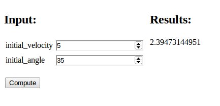
Flask interface

Flask is a tool that can be used to write a graphical user interface (GUI) to be operated in a web browser. Here we shall use Flask to create a GUI for our compute function, as displayed in Figure 1. To this end, simply create a Python file generate.py with the following lines:

from parampool.generator.flask import generate
from compute import compute_drag_free_landing

generate(compute_drag_free_landing, default_field='FloatField')

The generate function grabs the arguments in our compute function and creates the necessary Flask files.

Since the generate tool has no idea about the type of variable of the two positional arguments in the compute function, it has to assume some type. By default this will be text, but we can change that behavior to be floats by the setting the default_field argument to FloatField. This means that the generated interface will (only) accept float values for the input variables, which is sufficient in our case.

A graphical Flask-based web interface is generated by running

Terminal> python generate.py

You can now view the generated web interface by running

Terminal> python controller.py

and open your web browser at the location http://127.0.0.1:5000/. Fill in values for the two input variables and press Compute. The page in the Chrome browser will now look like Figure 1. Other browsers (Firefox, for instance) may have a slightly different design of the input fields. The figures in this tutorial were made with the Chrome and Opera browsers.

Django interface

Django is a very widespread and popular programming environment for creating web applications. We can easily create our web application in Django too. Just replace flask by django in generate.py:

from parampool.generator.django import generate
from compute import compute_drag_free_landing

generate(compute_drag_free_landing, default_field='FloatField')

The Django files are now in the directory tree drag_free_landing (same name as our compute function, except that any leading compute_ word is removed). Run the application by

Terminal> python drag_free_landing/manage.py runserver

and open your browser at the location http://127.0.0.1:8000/. The interface looks the same and has the same behavior as in the Flask example above.

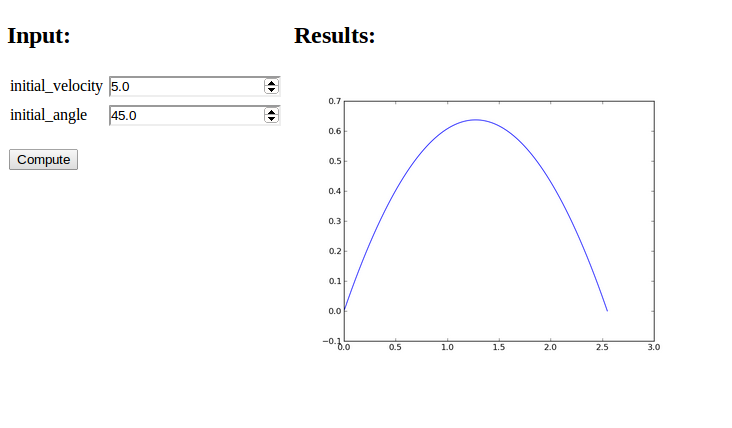
A plot as output

The result of the previous computation was just a number. Let us instead make a plot of the trajectory of a ball without any air resistance. The function

def compute_drag_free_motion_plot(
    initial_velocity=5.0,
    initial_angle=45.0):
    ...
    return html_text

is now our compute function, in compute.py, which takes the same two input arguments as before, but returns some HTML text that will display a plot in the browser window. This HTML text is basically the inclusion of the image file containing the plot,

<img src="X">

where X is the name of the file. However, if you do repeated computations, the name of the image file must change for the browser to update the plot. Inside the compute function we must therefore generate a unique name of each image file. For this purpose, we can use the number of seconds since the Epoch (January 1, 1970) as part of the filename, obtained by calling time.time(). In addition, the image file must reside in a subdirectory static. The appropriate code is displayed below.

import matplotlib.pyplot as plt
...
def compute_drag_free_motion_plot(
    initial_velocity=5.0,
    initial_angle=45.0):
    ...
    plt.plot(x, y)
    import time  # use time to make unique filenames
    filename = 'tmp_%s.png' % time.time()
    if not os.path.isdir('static'):
        os.mkdir('static')
    filename = os.path.join('static', filename)
    plt.savefig(filename)
    html_text = '<img src="%s" width="400">' % filename
    return html_text

The string version of the object returned from the compute function is inserted as Results in the HTML file, to the right of the input. By returning the appropriate HTML text the compute function can tailor the result part of the page to our needs.

Flask application

The generate.py file for this example is similar to what is shown above. Only the name of the compute function has changed:

from parampool.generator.flask import generate
from compute import compute_drag_free_motion_plot

generate(compute_drag_free_motion_plot)

We run python generator.py to generate the Flask files and then just writing python controller.py starts the web GUI. Now the default values appear in the input fields. These can be altered, or you can just click Compute. The computations result in a plot as showed in Figure 2.

Django application

The corresponding Django application is generated by the same generator.py code as above, except that the word flask is replaced by django. The Django files are now placed in the drag_free_motion_plot subdirectory, and the web GUI is started by running

Terminal> python drag_free_motion_plot/manage.py runserver

The functionality of the GUI is identical to that of the Flask version.

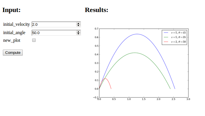
Comparing graphs in the same plot

With a little trick we can compare several trajectories in the same plot: inserting plt.figure(X) makes all plt.plot calls draw curves in the same figure (with figure number X). We introduce a boolean parameter new_plot reflecting whether we want a new fresh plot or not,

def compute_drag_free_motion_plot2(
    initial_velocity=5.0,
    initial_angle=45.0,
    new_plot=True):

and add the following code before the plt.plot call:

global fig_no
if new_plot:
    fig_no = plt.figure().number
else:
    plt.figure(fig_no)
plt.plot(x, y, label=r'$v=%g,\ \theta=%g$' %
         (initial_velocity, initial_angle))
plt.legend()

The new_plot parameter will turn up as a boolean variable in the web interface, and when checked, we create a new figure. Otherwise, we draw curves in the existing figure number fig_no which was initialized last time new_plot was true (with a global variable we ensure that the value of fig_no survives between the calls to the compute function). Figure 3 displays an attempt to not check new_plot and compare the curves corresponding to three different parameters (the files are in the flask3 directory.

if new_plot:
    fig_no = plt.figure().number
else:
    try:
        plt.figure(fig_no)
    except NameError:
        fig_no = plt.figure().number

import matplotlib.pyplot as plt
# make plot
from StringIO import StringIO
figfile = StringIO()
plt.savefig(figfile, format='png')
figfile.seek(0)  # rewind to beginning of file
figdata_png = figfile.buf  # extract string
import base64
figdata_png = base64.b64encode(figdata_png)
html_text = '<img src="data:image/png;base64,%s" width="400">' % \ 
            figdata_png

from parampool.utils import save_png_to_str
# make plot in plt (matplotlib.pyplot) object
html_text = save_png_to_str(plt, plotwidth=400)

<img src="data:image/png;base64,..." width="...">

import matplotlib as mpl
mpl.use('Agg')
import matplotlib.pyplot as plt

Bokeh plotting

One can use the Bokeh library for plotting instead of Matplotlib, see [1] for an example. The major problem is that Parampool generates the view.html file and the head and body parts of the HTML file generated by Bokeh must be inserted in the view.html file at the right places. This can be done manually or by a suitable script.

mpld3 plotting

The mpld3 library can be used to convert Matplotlib plots to a string containing all the HTML code for the plot:

# Plot array y vs x
import matplotlib.pyplot as plt, mpld3
fig, ax = plt.subplots()
ax.plot(x, y)
html_text = mpld3.fig_to_html(fig)

It is relatively easy to create interactive plots with mpld3.

Pandas highcharts plotting

The pandas-highcharts package is another strong and popular alternative for interative plotting in web pages.

More input parameters and results

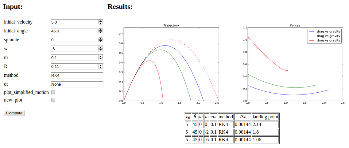
It is time to address a more complicated application: we want to compute the trajectory of a ball subject to air drag and lift and compare that trajectory to the one where drag and lift are omitted. We also want to visualize the relative importance between the three forces: gravity, drag, and lift. The lift is caused by spinning the ball.

The function that performs the computations has the following signature:

def compute_motion_and_forces0(
    initial_velocity=5.0,
    initial_angle=45.0,
    spinrate=50.0,
    w=0.0,
    m=0.1,
    R=0.11,
    method='RK4',
    dt=None,
    plot_simplified_motion=True,
    new_plot=True
    ):

and returns a formatted string html_text with two plots organized in an HTML table.

The returned HTML code

The technique described in the Avoiding plot files box at the end of the section A plot as output is implemented to embed PNG images directly in the HTML code. Under the plots there is a table of input values and the landing point. Curves can be accumulated in the plots (new_plot=True), with the corresponding data added to the table. A rough sketch of the HTML code returned from the compute function goes as follows:

<table>
<tr>
<td valign="top">
<img src="data:image/png;base64,iVBORw0KGgoAAAA..." width="400">
</td>
<td valign="top">
<img src="data:image/png;base64,iVBORw0KGgoAAAA..." width="400">
</td>
</tr>
</table>

<center>
<table border=1>
<tr>
<td align="center"> \( v_0 \)  </td>
<td align="center"> \( \theta \) </td>
<td align="center"> \( \omega \) </td>
<td align="center"> \( w \)    </td>
<td align="center"> \( m \)    </td>
<td align="center"> \( R \)    </td>
<td align="center"> method     </td>
<td align="center"> \( \Delta t \) </td>
<td align="center"> landing point </td>
</tr>
<tr><td align="right"> 5 </td><td align="right"> 45 </td> ...</tr>
<tr><td align="right"> 5 </td><td align="right"> 45 </td> ...</tr>
<tr><td align="right"> 5 </td><td align="right"> 45 </td> ...</tr>
</table>
</center>

Note that we use MathJax syntax for having LaTeX mathematics in the table heading. All details about the computations and the construction of the returned HTML string can be found in the compute.py file.

Documentation of the application

The Parampool generate function applies the convention that any doc string of the compute function is copied and typeset verbatim at the top of the web interface. However, if the text # (DocOnce format) appears somewhere in the doc string, the text is taken as DocOnce source code and translated to HTML, which enables typesetting of LaTeX mathematics and computer code snippets (with nice pygments formatting).

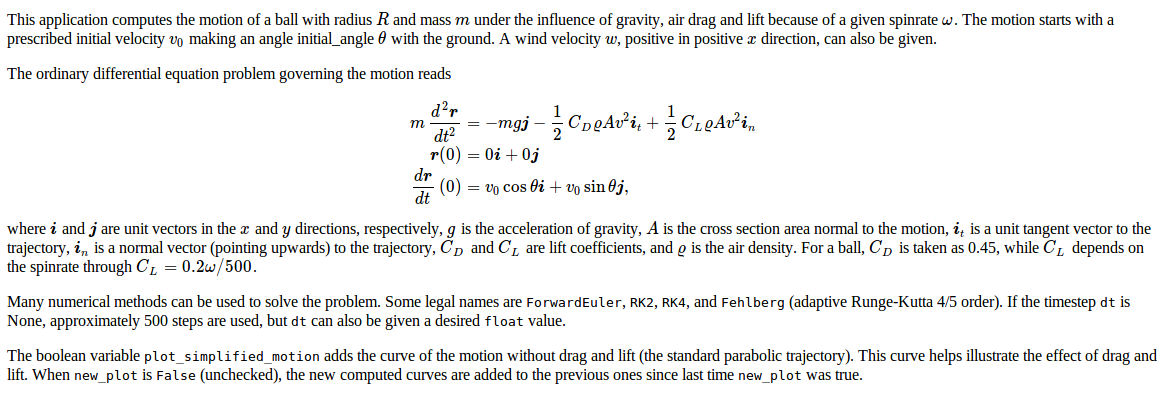
The documentation of the web interface can therefore be included as a doc string in the compute function. Here is descriptive doc string using DocOnce syntax for LaTeX mathematics (equations inside !bt and !et commands) and monospace font for Python variables (names in backticks). The corresponding view in a browser is shown in Figure 5.

"""
This application computes the motion of a ball with radius $R$
and mass $m$ under the influence of gravity, air drag and lift
because of a given spinrate $\omega$. The motion starts with a
prescribed initial velocity $v_0$ making an angle initial_angle
$\theta$ with the ground. A wind velocity $w$, positive in
positive $x$ direction, can also be given.

The ordinary differential equation problem governing the
motion reads

!bt
\begin{align*}
m\frac{d^2\boldsymbol{r}}{dt^2} &= -mg\boldsymbol{j} -
\frac{1}{2}C_D\varrho A v^2\boldsymbol{i}_t +
\frac{1}{2}C_L\varrho A v^2\boldsymbol{i}_n\\ 
\boldsymbol{r}(0) &= 0\boldsymbol{i} + 0\boldsymbol{j}\\ 
\frac{d\boldsymbol{r}}{dt}(0) &= v_0\cos\theta\boldsymbol{i} + v_0\sin\theta\boldsymbol{j},
\end{align*}
!et
where $\boldsymbol{i}$ and $\boldsymbol{j}$ are unit vectors in the $x$ and $y$
directions, respectively, $g$ is the acceleration of gravity,
$A$ is the cross section area normal to the motion, $\boldsymbol{i}_t$
is a unit tangent vector to the trajectory, $\boldsymbol{i}_n$ is
a normal vector (pointing upwards) to the trajectory,
$C_D$ and $C_L$ are lift coefficients, and $\varrho$ is the
air density. For a ball, $C_D$ is taken as 0.45, while
$C_L$ depends on the spinrate through $C_L=0.2\omega/500$.

Many numerical methods can be used to solve the problem.
Some legal names are `ForwardEuler`, `RK2`, `RK4`,
and `Fehlberg` (adaptive Runge-Kutta 4/5 order).  If the
timestep `dt` is None, approximately 500 steps are used, but
`dt` can also be given a desired `float` value.

The boolean variable `plot_simplified_motion` adds the curve
of the motion without drag and lift (the standard parabolic
trajectory). This curve helps illustrate the effect of drag
and lift. When `new_plot` is `False` (unchecked), the new
computed curves are added to the previous ones since last
time `new_plot` was true.

# (DocOnce format)
"""

The generate.py code for creating the web GUI goes as in the other examples,

from parampool.generator.flask import generate
from compute import compute_motion_and_forces

generate(compute_motion_and_forces, MathJax=True)

and we start the application as usual by python controller.py. The resulting web interface appears in Figure 4. The table shows the sequence of data we have given; starting with the default values, then turning off the plot_simplified_motion curve and new_plot, then running two cases with different values for the wind parameter w. The plot clearly show the influence of drag and wind against the motion.

Django interface

As before, the Django interface is generated by importing the function generate from parampool.generator.django. A subdirectory motion_and_forces contains the files, and the Django application is started as shown in previous examples and has the same functionality as the Flask application.

Other types of input data

The generate function will recognize the following different types of keyword arguments in the compute function: float, int, bool, str, list, tuple, numpy.ndarray, name of a file, as well as user-defined class types (a la MyClass).

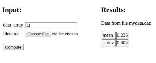
Uploading a file

Here is a minimalistic example on computing the mean and standard deviation of data either in an array or in a file (we use the file if the operator of the web interface assigns a name in the "filename" entry):

def compute_average(data_array=np.array([1]), filename=None):
    if filename is not None:
        data = np.loadtxt(os.path.join('uploads', filename))
        what = 'file %s' % filename
    else:
        data = data_array
        what = 'data_array'
    return """
Data from %s:
<p>
<table border=1>
<tr><td> mean    </td><td> %.3g </td></tr>
<tr><td> st.dev. </td><td> %.3g </td></tr>
</table></p>
""" % (what, np.mean(data), np.std(data))

The output is simple, basically two numbers in a table and an intro line.

We write a generate.py file as shown before, but with compute_average as the name of the compute function. For any argument containing the string filename it is assumed that the argument represents the name of a file. The web interface will then feature a button for uploading the file.

When the application runs, we have two data fields: one for setting an array with list syntax and one for uploading a file. Clicking on the latter and uploading a file mydata.dat containing just columns of numbers, results in the web page displayed in Figure 6. In this case, when a filename was assigned, we use the data in the file. Alternatively, we can instead fill in the data array and click Compute, which then will compute the basic statistics of the assigned data array.

• «
• 1
• 2
• 3
• 4
• 5
• 6
• 7
• »