Implementation (3)

We shall now describe in detail various Python implementations for solving a standard 2D, linear wave equation with constant wave velocity and \(u=0\) on the boundary. The wave equation is to be solved in the space-time domain \(\Omega\times (0,T]\), where \(\Omega = (0,L_x)\times (0,L_y)\) is a rectangular spatial domain. More precisely, the complete initial-boundary value problem is defined by

\[u_t = c^2(u_{xx} + u_{yy}) + f(x,y,t),\quad (x,y)\in \Omega,\ t\in (0,T],\]

\[u(x,y,0) = I(x,y),\quad (x,y)\in\Omega,\]

\[u_t(x,y,0) = V(x,y),\quad (x,y)\in\Omega,\]

\[u = 0,\quad (x,y)\in\partial\Omega,\ t\in (0,T],\]

where \(\partial\Omega\) is the boundary of \(\Omega\), in this case the four sides of the rectangle \([0,L_x]\times [0,L_y]\): \(x=0\), \(x=L_x\), \(y=0\), and \(y=L_y\).

The PDE is discretized as

\[[D_t D_t u = c^2(D_xD_x u + D_yD_y u) + f]^n_{i,j},\]

which leads to an explicit updating formula to be implemented in a program:

\[u^{n+1} = -u^{n-1}_{i,j} + 2u^n_{i,j} + \nonumber\]

(1)\[ \quad C_x^2( u^{n}_{i+1,j} - 2u^{n}_{i,j} + u^{n}_{i-1,j}) + C_y^2 (u^{n}_{i,j+1} - 2u^{n}_{i,j} + u^{n}_{i,j-1}) + \Delta t^2 f_{i,j}^n,\]

for all interior mesh points \(i\in{{\mathcal{I^i}_x}}\) and \(j\in{{\mathcal{I^i}_y}}\), and for \(n\in{{\mathcal{I^+}_t}}\). The constants \(C_x\) and \(C_y\) are defined as

\[C_x = c\frac{\Delta t}{\Delta x},\quad C_x = c\frac{\Delta t}{\Delta y} {\thinspace .}\]

At the boundary we simply set \(u^{n+1}_{i,j}=0\) for \(i=0\), \(j=0,\ldots,N_y\); \(i=N_x\), \(j=0,\ldots,N_y\); \(j=0\), \(i=0,\ldots,N_x\); and \(j=N_y\), \(i=0,\ldots,N_x\). For the first step, \(n=0\), (2) is combined with the discretization of the initial condition \(u_t=V\), \([D_{2t} u = V]^0_{i,j}\) to obtain a special formula for \(u^1_{i,j}\) at the interior mesh points:

\[u^{1} = u^0_{i,j} + \Delta t V_{i,j} + \nonumber\]

(2)\[ \quad {\frac{1}{2}}C_x^2( u^{0}_{i+1,j} - 2u^{0}_{i,j} + u^{0}_{i-1,j}) + {\frac{1}{2}}C_y^2 (u^{0}_{i,j+1} - 2u^{0}_{i,j} + u^{0}_{i,j-1}) + \frac{1}{2}\Delta t^2f_{i,j}^n,\]

The algorithm is very similar to the one in 1D:

1. Set initial condition \(u^0_{i,j}=I(x_i,y_j)\)
2. Compute \(u^1_{i,j}\) from (2)
3. Set \(u^1_{i,j}=0\) for the boundaries \(i=0,N_x\), \(j=0,N_y\)
4. For \(n=1,2,\ldots,N_t\):

1. Find \(u^{n+1}_{i,j}\) from (2) for all internal mesh points, \(i\in{{\mathcal{I^i}_x}}\), \(j\in{{\mathcal{I^i}_y}}\)
2. Set \(u^{n+1}_{i,j}=0\) for the boundaries \(i=0,N_x\), \(j=0,N_y\)

Scalar computations

The solver function for a 2D case with constant wave velocity and \(u=0\) as boundary condition follows the setup from the similar function for the 1D case in wave1D_u0_s.py, but there are a few necessary extensions. The code is in the program wave2D_u0.py.

Domain and mesh

The spatial domain is now \([0,L_x]\times [0,L_y]\), specified by the arguments Lx and Ly. Similarly, the number of mesh points in the \(x\) and \(y\) directions, \(N_x\) and \(N_y\), become the arguments Nx and Ny. In multi-dimensional problems it makes less sense to specify a Courant number as the wave velocity is a vector and the mesh spacings may differ in the various spatial directions. We therefore give \(\Delta t\) explicitly. The signature of the solver function is then

def solver(I, V, f, c, Lx, Ly, Nx, Ny, dt, T,
           user_action=None, version='scalar'):

Key parameters used in the calculations are created as

x = linspace(0, Lx, Nx+1)                  # mesh points in x dir
y = linspace(0, Ly, Ny+1)                  # mesh points in y dir
dx = x[1] - x[0]
dy = y[1] - y[0]
Nt = int(round(T/float(dt)))
t = linspace(0, N*dt, N+1)                 # mesh points in time
Cx2 = (c*dt/dx)**2;  Cy2 = (c*dt/dy)**2    # help variables
dt2 = dt**2

Solution arrays

We store \(u^{n+1}_{i,j}\), \(u^{n}_{i,j}\), and \(u^{n-1}_{i,j}\) in three two-dimensional arrays,

u   = zeros((Nx+1,Ny+1))   # solution array
u_1 = zeros((Nx+1,Ny+1))   # solution at t-dt
u_2 = zeros((Nx+1,Ny+1))   # solution at t-2*dt

where \(u^{n+1}_{i,j}\) corresponds to u[i,j], \(u^{n}_{i,j}\) to u_1[i,j], and \(u^{n-1}_{i,j}\) to u_2[i,j]

Index sets

It is also convenient to introduce the index sets (cf. The section Index set notation)

Ix = range(0, u.shape[0])
Iy = range(0, u.shape[1])
It = range(0, t.shape[0])

Computing the solution

Inserting the initial condition I in u_1 and making a callback to the user in terms of the user_action function is a straightforward generalization of the 1D code from the section Sketch of an implementation:

for i in Ix:
    for j in Iy:
        u_1[i,j] = I(x[i], y[j])

if user_action is not None:
    user_action(u_1, x, xv, y, yv, t, 0)

The user_action function has additional arguments compared to the 1D case. The arguments xv and yv fact will be commented upon in the section Vectorized computations.

The key finite difference formula (6.5) for updating the solution at a time level is implemented in a separate function as

def advance_scalar(u, u_1, u_2, f, x, y, t, n, Cx2, Cy2, dt,
                   V=None, step1=False):
    Ix = range(0, u.shape[0]);  Iy = range(0, u.shape[1])
    dt2 = dt**2
    if step1:
        Cx2 = 0.5*Cx2;  Cy2 = 0.5*Cy2; dt2 = 0.5*dt2
        D1 = 1;  D2 = 0
    else:
        D1 = 2;  D2 = 1
    for i in Ix[1:-1]:
        for j in Iy[1:-1]:
            u_xx = u_1[i-1,j] - 2*u_1[i,j] + u_1[i+1,j]
            u_yy = u_1[i,j-1] - 2*u_1[i,j] + u_1[i,j+1]
            u[i,j] = D1*u_1[i,j] - D2*u_2[i,j] + \
                     Cx2*u_xx + Cy2*u_yy + dt2*f(x[i], y[j], t[n])
            if step1:
                u[i,j] += dt*V(x[i], y[j])
    # Boundary condition u=0
    j = Iy[0]
    for i in Ix: u[i,j] = 0
    j = Iy[-1]
    for i in Ix: u[i,j] = 0
    i = Ix[0]
    for j in Iy: u[i,j] = 0
    i = Ix[-1]
    for j in Iy: u[i,j] = 0
    return u

The step1 variable has been introduced to allow the formula to be reused for first step \(u^1_{i,j}\):

u = advance_scalar(u, u_1, u_2, f, x, y, t,
                   n, Cx2, Cy2, dt, V, step1=True)

Below, we will make many alternative implementations of the advance_scalar function to speed up the code since most of the CPU time in simulations is spent in this function.

Vectorized computations

The scalar code above turns out to be extremely slow for large 2D meshes, and probably useless in 3D beyond debugging of small test cases. Vectorization is therefore a must for multi-dimensional finite difference computations in Python. For example, with a mesh consisting of \(30\times 30\) cells, vectorization brings down the CPU time by a factor of 70 (!).

In the vectorized case we must be able to evaluate user-given functions like \(I(x,y)\) and \(f(x,y,t)\), provided as Python functions I(x,y) and f(x,y,t), for the entire mesh in one array operation. Having the one-dimensional coordinate arrays x and y is not sufficient: these must be extended to vectorized versions,

from numpy import newaxis
xv = x[:,newaxis]
yv = y[newaxis,:]
# or
xv = x.reshape((x.size, 1))
yv = y.reshape((1, y.size))

This is a standard required technique when evaluating functions over a 2D mesh, say sin(xv)*cos(xv), which then gives a result with shape (Nx+1,Ny+1).

With the xv and yv arrays for vectorized computing, setting the initial condition is just a matter of

u_1[:,:] = I(xv, yv)

One could also have written u_1 = I(xv, yv) and let u_1 point to a new object, but vectorized operations often makes use of direct insertion in the original array through u_1[:,:] because sometimes not all of the array is to be filled by such a function evaluation. This is the case with the computational scheme for \(u^{n+1}_{i,j}\):

def advance_vectorized(u, u_1, u_2, f_a, Cx2, Cy2, dt,
                       V=None, step1=False):
    dt2 = dt**2
    if step1:
        Cx2 = 0.5*Cx2;  Cy2 = 0.5*Cy2; dt2 = 0.5*dt2
        D1 = 1;  D2 = 0
    else:
        D1 = 2;  D2 = 1
    u_xx = u_1[:-2,1:-1] - 2*u_1[1:-1,1:-1] + u_1[2:,1:-1]
    u_yy = u_1[1:-1,:-2] - 2*u_1[1:-1,1:-1] + u_1[1:-1,2:]
    u[1:-1,1:-1] = D1*u_1[1:-1,1:-1] - D2*u_2[1:-1,1:-1] + \
                   Cx2*u_xx + Cy2*u_yy + dt2*f_a[1:-1,1:-1]
    if step1:
        u[1:-1,1:-1] += dt*V[1:-1, 1:-1]
    # Boundary condition u=0
    j = 0
    u[:,j] = 0
    j = u.shape[1]-1
    u[:,j] = 0
    i = 0
    u[i,:] = 0
    i = u.shape[0]-1
    u[i,:] = 0
    return u

Array slices in 2D are more complicated to understand than those in 1D, but the logic from 1D applies to each dimension separately. For example, when doing \(u^{n}_{i,j} - u^{n}_{i-1,j}\) for \(i\in{{\mathcal{I^+}_x}}\), we just keep j constant and make a slice in the first index: u_1[1:,j] - u_1[:-1,j], exactly as in 1D. The 1: slice specifies all the indices \(i=1,2,\ldots,N_x\) (up to the last valid index), while :-1 specifies the relevant indices for the second term: \(0,1,\ldots,N_x-1\) (up to, but not including the last index).

In the above code segment, the situation is slightly more complicated, because each displaced slice in one direction is accompanied by a 1:-1 slice in the other direction. The reason is that we only work with the internal points for the index that is kept constant in a difference.

The boundary conditions along the four sides makes use of a slice consisting of all indices along a boundary:

u[: ,0] = 0
u[:,Ny] = 0
u[0 ,:] = 0
u[Nx,:] = 0

The f function is in the above vectorized update of u first computed as an array over all mesh points:

f_a = f(xv, yv, t[n])

We could, alternatively, used the call f(xv, yv, t[n])[1:-1,1:-1] in the last term of the update statement, but other implementations in compiled languages benefit from having f available in an array rather than calling our Python function f(x,y,t) for every point.

Also in the advance_vectorized function we have introduced a boolean step1 to reuse the formula for the first time step in the same way as we did with advance_scalar. We refer to the solver function in wave2D_u0.py for the details on how the overall algorithm is implemented.

The callback function now has the arguments u, x, xv, y, yv, t, n. The inclusion of xv and yv makes it easy to, e.g., compute an exact 2D solution in the callback function and compute errors, through an expression like u - exact_solution(xv, yv, t[n]).

Verification (3)

Testing a quadratic solution

The 1D solution from the section Constructing an exact solution of the discrete equations can be generalized to multi-dimensions and provides a test case where the exact solution also fulfills the discrete equations such that we know (to machine precision) what numbers the solver function should produce. In 2D we use the following generalization of (2.21):

(3)\[ {u_{\small\mbox{e}}}(x,y,t) = x(L_x-x)y(L_y-y)(1+{\frac{1}{2}}t) {\thinspace .}\]

This solution fulfills the PDE problem if \(I(x,y)={u_{\small\mbox{e}}}(x,y,0)\), \(V=\frac{1}{2}{u_{\small\mbox{e}}}(x,y,0)\), and \(f=2c^2(1+{\frac{1}{2}}t)(y(L_y-y) + x(L_x-x))\). To show that \({u_{\small\mbox{e}}}\) also solves the discrete equations, we start with the general results \([D_t D_t 1]^n=0\), \([D_t D_t t]^n=0\), and \([D_t D_t t^2]=2\), and use these to compute

\[[D_xD_x {u_{\small\mbox{e}}}]^n_{i,j} = [y(L_y-y)(1+{\frac{1}{2}}t) D_xD_x x(L_x-x)]^n_{i,j} = y_j(L_y-y_j)(1+{\frac{1}{2}}t_n)2{\thinspace .}\]

A similar calculation must be carried out for the \([D_yD_y {u_{\small\mbox{e}}}]^n_{i,j}\) and \([D_tD_t {u_{\small\mbox{e}}}]^n_{i,j}\) terms. One must also show that the quadratic solution fits the special formula for \(u^1_{i,j}\). The details are left as Exercise 10: Check that a solution fulfills the discrete model. The test_quadratic function in the wave2D_u0.py program implements this verification as a nose test.

Migrating loops to Cython

Although vectorization can bring down the CPU time dramatically compared with scalar code, there is still some factor 5-10 to win in these types of applications by implementing the finite difference scheme in compiled code, typically in Fortran, C, or C++. This can quite easily be done by adding a little extra code to our program. Cython is an extension of Python that offers the easiest way to nail our Python loops in the scalar code down to machine code and the efficiency of C.

Cython can be viewed as an extended Python language where variables are declared with types and where functions are marked to be implemented in C. Migrating Python code to Cython is done by copying the desired code segments to functions (or classes) and placing them in one or more separate files with extension .pyx.

Declaring variables and annotating the code

Our starting point is the plain advance_scalar function for a scalar implementation of the updating algorithm for new values \(u^{n+1}_{i,j}\):

def advance_scalar(u, u_1, u_2, f, x, y, t, n, Cx2, Cy2, dt,
                   V=None, step1=False):
    Ix = range(0, u.shape[0]);  Iy = range(0, u.shape[1])
    dt2 = dt**2
    if step1:
        Cx2 = 0.5*Cx2;  Cy2 = 0.5*Cy2; dt2 = 0.5*dt2
        D1 = 1;  D2 = 0
    else:
        D1 = 2;  D2 = 1
    for i in Ix[1:-1]:
        for j in Iy[1:-1]:
            u_xx = u_1[i-1,j] - 2*u_1[i,j] + u_1[i+1,j]
            u_yy = u_1[i,j-1] - 2*u_1[i,j] + u_1[i,j+1]
            u[i,j] = D1*u_1[i,j] - D2*u_2[i,j] + \
                     Cx2*u_xx + Cy2*u_yy + dt2*f(x[i], y[j], t[n])
            if step1:
                u[i,j] += dt*V(x[i], y[j])
    # Boundary condition u=0
    j = Iy[0]
    for i in Ix: u[i,j] = 0
    j = Iy[-1]
    for i in Ix: u[i,j] = 0
    i = Ix[0]
    for j in Iy: u[i,j] = 0
    i = Ix[-1]
    for j in Iy: u[i,j] = 0
    return u

We simply take a copy of this function and put it in a file wave2D_u0_loop_cy.pyx. The relevant Cython implementation arises from declaring variables with types and adding some important annotations to speed up array computing in Cython. Let us first list the complete code in the .pyx file:

import numpy as np
cimport numpy as np
cimport cython
ctypedef np.float64_t DT    # data type

@cython.boundscheck(False)  # turn off array bounds check
@cython.wraparound(False)   # turn off negative indices (u[-1,-1])
cpdef advance(
    np.ndarray[DT, ndim=2, mode='c'] u,
    np.ndarray[DT, ndim=2, mode='c'] u_1,
    np.ndarray[DT, ndim=2, mode='c'] u_2,
    np.ndarray[DT, ndim=2, mode='c'] f,
    double Cx2, double Cy2, double dt2):

    cdef int Ix_start = 0
    cdef int Iy_start = 0
    cdef int Ix_end = u.shape[0]-1
    cdef int Iy_end = u.shape[1]-1
    cdef int i, j
    cdef double u_xx, u_yy

    for i in range(Ix_start+1, Ix_end):
        for j in range(Iy_start+1, Iy_end):
            u_xx = u_1[i-1,j] - 2*u_1[i,j] + u_1[i+1,j]
            u_yy = u_1[i,j-1] - 2*u_1[i,j] + u_1[i,j+1]
            u[i,j] = 2*u_1[i,j] - u_2[i,j] + \
                     Cx2*u_xx + Cy2*u_yy + dt2*f[i,j]
    # Boundary condition u=0
    j = Iy_start
    for i in range(Ix_start, Ix_end+1): u[i,j] = 0
    j = Iy_end
    for i in range(Ix_start, Ix_end+1): u[i,j] = 0
    i = Ix_start
    for j in range(Iy_start, Iy_end+1): u[i,j] = 0
    i = Iy_end
    for j in range(Iy_start, Iy_end+1): u[i,j] = 0
    return u

This example may act as a recipe on how to transform array-intensive code with loops into Cython.

1. Variables are declared with types: for example, double v in the argument list instead of just v, and cdef double v for a variable v in the body of the function. A Python float object is declared as double for translation to C by Cython, while an int object is declared by int.
2. Arrays need a comprehensive type declaration involving
   • the type np.ndarray,
   • the data type of the elements, here 64-bit floats, abbreviated as DT through ctypedef np.float64_t DT (instead of DT we could use the full name of the data type: np.float64_t, which is a Cython-defined type),
   • the dimensions of the array, here ndim=2 and ndim=1,
   • specification of contiguous memory for the array (mode='c').
3. Functions declared with cpdef are translated to C but also accessible from Python.
4. In addition to the standard numpy import we also need a special Cython import of numpy: cimport numpy as np, to appear after the standard import.
5. By default, array indices are checked to be within their legal limits. To speed up the code one should turn off this feature for a specific function by placing @cython.boundscheck(False) above the function header.
6. Also by default, array indices can be negative (counting from the end), but this feature has a performance penalty and is therefore here turned off by writing @cython.wraparound(False) right above the function header.
7. The use of index sets Ix and Iy in the scalar code cannot be successfully translated to C. One reason is that constructions like Ix[1:-1] involve negative indices, and these are now turned off. Another reason is that Cython loops must take the form for i in xrange or for i in range for being translated into efficient C loops. We have therefore introduced Ix_start as Ix[0] and Ix_end as Ix[-1] to hold the start and end of the values of index \(i\). Similar variables are introduced for the \(j\) index. A loop for i in Ix is with these new variables written as for i in range(Ix_start, Ix_end+1).

Array declaration syntax in Cython

We have used the syntax np.ndarray[DT, ndim=2, mode='c'] to declare numpy arrays in Cython. There is a simpler, alternative syntax, employing typed memory views, where the declaration looks like double [:,:]. However, the full support for this functionality is not yet ready, and in this text we use the full array declaration syntax.

Visual inspection of the C translation

Cython can visually explain how successfully it can translate a code from Python to C. The command

Terminal> cython -a wave2D_u0_loop_cy.pyx

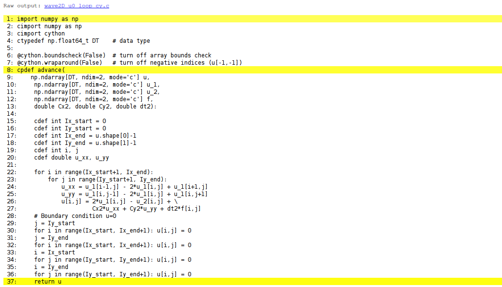
produces an HTML file wave2D_u0_loop_cy.html, which can be loaded into a web browser to illustrate which lines of the code that have been translated to C. Figure Visual illustration of Cython’s ability to translate Python to C shows the illustrated code. Yellow lines indicate the lines that Cython did not manage to translate to efficient C code and that remain in Python. For the present code we see that Cython is able to translate all the loops with array computing to C, which is our primary goal.

Visual illustration of Cython’s ability to translate Python to C

You can also inspect the generated C code directly, as it appears in the file wave2D_u0_loop_cy.c. Nevertheless, understanding this C code requires some familiarity with writing Python extension modules in C by hand. Deep down in the file we can see in detail how the compute-intensive statements are translated some complex C code that is quite different from what we a human would write (at least if a direct correspondence to the mathematics was in mind).

Building the extension module (1)

Cython code must be translated to C, compiled, and linked to form what is known in the Python world as a C extension module. This is usually done by making a setup.py script, which is the standard way of building and installing Python software. For an extension module arising from Cython code, the following setup.py script is all we need to build and install the module:

from distutils.core import setup
from distutils.extension import Extension
from Cython.Distutils import build_ext

cymodule = 'wave2D_u0_loop_cy'
setup(
  name=cymodule
  ext_modules=[Extension(cymodule, [cymodule + '.pyx'],)],
  cmdclass={'build_ext': build_ext},
)

We run the script by

Terminal> python setup.py build_ext --inplace

The --inplace option makes the extension module available in the current directory as the file wave2D_u0_loop_cy.so. This file acts as a normal Python module that can be imported and inspected:

>>> import wave2D_u0_loop_cy
>>> dir(wave2D_u0_loop_cy)
['__builtins__', '__doc__', '__file__', '__name__',
 '__package__', '__test__', 'advance', 'np']

The important output from the dir function is our Cython function advance (the module also features the imported numpy module under the name np as well as many standard Python objects with double underscores in their names).

The setup.py file makes use of the distutils package in Python and Cython’s extension of this package. These tools know how Python was built on the computer and will use compatible compiler(s) and options when building other code in Cython, C, or C++. Quite some experience with building large program systems is needed to do the build process manually, so using a setup.py script is strongly recommended.

Simplified build of a Cython module

When there is no need to link the C code with special libraries, Cython offers a shortcut for generating and importing the extension module:

import pyximport; pyximport.install()

This makes the setup.py script redundant. However, in the wave2D_u0.py code we do not use pyximport and require an explicit build process of this and many other modules.

Calling the Cython function from Python

The wave2D_u0_loop_cy module contains our advance function, which we now may call from the Python program for the wave equation:

import wave2D_u0_loop_cy
advance = wave2D_u0_loop_cy.advance
...
for n in It[1:-1:                  # time loop
    f_a[:,:] = f(xv, yv, t[n])     # precompute, size as u
    u = advance(u, u_1, u_2, f_a, x, y, t, Cx2, Cy2, dt2)

Efficiency (1)

For a mesh consisting of \(120\times 120\) cells, the scalar Python code require 1370 CPU time units, the vectorized version requires 5.5, while the Cython version requires only 1! For a smaller mesh with \(60\times 60\) cells Cython is about 1000 times faster than the scalar Python code, and the vectorized version is about 6 times slower than the Cython version.

Migrating loops to Fortran

Instead of relying on Cython’s (excellent) ability to translate Python to C, we can invoke a compiled language directly and write the loops ourselves. Let us start with Fortran 77, because this is a language with more convenient array handling than C (or plain C++). Or more precisely, we can with ease program with the same multi-dimensional indices in the Fortran code as in the numpy arrays in the Python code, while in C these arrays are one-dimensional and requires us to reduce multi-dimensional indices to a single index.

The Fortran subroutine

We write a Fortran subroutine advance in a file wave2D_u0_loop_f77.f for implementing the updating formula (2) and setting the solution to zero at the boundaries:

      subroutine advance(u, u_1, u_2, f, Cx2, Cy2, dt2, Nx, Ny)
      integer Nx, Ny
      real*8 u(0:Nx,0:Ny), u_1(0:Nx,0:Ny), u_2(0:Nx,0:Ny)
      real*8 f(0:Nx, 0:Ny), Cx2, Cy2, dt2
      integer i, j
Cf2py intent(in, out) u

C     Scheme at interior points
      do j = 1, Ny-1
         do i = 1, Nx-1
            u(i,j) = 2*u_1(i,j) - u_2(i,j) +
     &      Cx2*(u_1(i-1,j) - 2*u_1(i,j) + u_1(i+1,j)) +
     &      Cy2*(u_1(i,j-1) - 2*u_1(i,j) + u_1(i,j+1)) +
     &      dt2*f(i,j)
         end do
      end do

C     Boundary conditions
      j = 0
      do i = 0, Nx
         u(i,j) = 0
      end do
      j = Ny
      do i = 0, Nx
         u(i,j) = 0
      end do
      i = 0
      do j = 0, Ny
         u(i,j) = 0
      end do
      i = Nx
      do j = 0, Ny
         u(i,j) = 0
      end do
      return
      end

This code is plain Fortran 77, except for the special Cf2py comment line, which here specifies that u is both an input argument and an object to be returned from the advance routine. Or more precisely, Fortran is not able return an array from a function, but we need a wrapper code in C for the Fortran subroutine to enable calling it from Python, and in this wrapper code one can return u to the calling Python code.

Remark

It is not strictly necessary to return u to the calling Python code since the advance function will modify the elements of u, but the convention in Python is to get all output from a function as returned values. That is, the right way of calling the above Fortran subroutine from Python is

u = advance(u, u_1, u_2, f, Cx2, Cy2, dt2)

The less encouraged style, which works and resembles the way the Fortran subroutine is called from Fortran, reads

advance(u, u_1, u_2, f, Cx2, Cy2, dt2)

Building the Fortran module with f2py

The nice feature of writing loops in Fortran is that the tool f2py can with very little work produce a C extension module such that we can call the Fortran version of advance from Python. The necessary commands to run are

Terminal> f2py -m wave2D_u0_loop_f77 -h wave2D_u0_loop_f77.pyf \
          --overwrite-signature wave2D_u0_loop_f77.f
Terminal> f2py -c wave2D_u0_loop_f77.pyf --build-dir build_f77 \
          -DF2PY_REPORT_ON_ARRAY_COPY=1 wave2D_u0_loop_f77.f

The first command asks f2py to interpret the Fortran code and make a Fortran 90 specification of the extension module in the file wave2D_u0_loop_f77.pyf. The second command makes f2py generate all necessary wrapper code, compile our Fortran file and the wrapper code, and finally build the module. The build process takes place in the specified subdirectory build_f77 so that files can be inspected if something goes wrong. The option -DF2PY_REPORT_ON_ARRAY_COPY=1 makes f2py write a message for every array that is copied in the communication between Fortran and Python, which is very useful for avoiding unnecessary array copying (see below). The name of the module file is wave2D_u0_loop_f77.so, and this file can be imported and inspected as any other Python module:

>>> import wave2D_u0_loop_f77
>>> dir(wave2D_u0_loop_f77)
['__doc__', '__file__', '__name__', '__package__',
 '__version__', 'advance']
>>> print wave2D_u0_loop_f77.__doc__
This module 'wave2D_u0_loop_f77' is auto-generated with f2py....
Functions:
  u = advance(u,u_1,u_2,f,cx2,cy2,dt2,
      nx=(shape(u,0)-1),ny=(shape(u,1)-1))

Examine the doc strings

Printing the doc strings of the module and its functions is extremely important after having created a module with f2py, because f2py makes Python interfaces to the Fortran functions that are different from how the functions are declared in the Fortran code (!). The rationale for this behavior is that f2py creates Pythonic interfaces such that Fortran routines can be called in the same way as one calls Python functions. Output data from Python functions is always returned to the calling code, but this is technically impossible in Fortran. Also, arrays in Python are passed to Python functions without their dimensions because that information is packed with the array data in the array objects, but this is not possible in Fortran. Therefore, f2py removes array dimensions from the argument list, and f2py makes it possible to return objects back to Python.

Let us follow the advice of examining the doc strings and take a close look at the documentation f2py has generated for our Fortran advance subroutine:

>>> print wave2D_u0_loop_f77.advance.__doc__
This module 'wave2D_u0_loop_f77' is auto-generated with f2py
Functions:
  u = advance(u,u_1,u_2,f,cx2,cy2,dt2,
              nx=(shape(u,0)-1),ny=(shape(u,1)-1))
.
advance - Function signature:
  u = advance(u,u_1,u_2,f,cx2,cy2,dt2,[nx,ny])
Required arguments:
  u : input rank-2 array('d') with bounds (nx + 1,ny + 1)
  u_1 : input rank-2 array('d') with bounds (nx + 1,ny + 1)
  u_2 : input rank-2 array('d') with bounds (nx + 1,ny + 1)
  f : input rank-2 array('d') with bounds (nx + 1,ny + 1)
  cx2 : input float
  cy2 : input float
  dt2 : input float
Optional arguments:
  nx := (shape(u,0)-1) input int
  ny := (shape(u,1)-1) input int
Return objects:
  u : rank-2 array('d') with bounds (nx + 1,ny + 1)

Here we see that the nx and ny parameters declared in Fortran are optional arguments that can be omitted when calling advance from Python.

We strongly recommend to print out the documentation of every Fortran function to be called from Python and make sure the call syntax is exactly as listed in the documentation.

How to avoid array copying

Multi-dimensional arrays are stored as a stream of numbers in memory. For a two-dimensional array consisting of rows and columns there are two ways of creating such a stream: row-major ordering, which means that rows are stored consecutively in memory, or column-major ordering, which means that the columns are stored one after each other. All programming languages inherited from C, including Python, apply the row-major ordering, but Fortran uses column-major storage. Thinking of a two-dimensional array in Python or C as a matrix, it means that Fortran works with the transposed matrix.

Fortunately, f2py creates extra code so that accessing u(i,j) in the Fortran subroutine corresponds to the element u[i,j] in the underlying numpy array (without the extra code, u(i,j) in Fortran would access u[j,i] in the numpy array). Technically, f2py takes a copy of our numpy array and reorders the data before sending the array to Fortran. Such copying can be costly. For 2D wave simulations on a \(60\times 60\) grid the overhead of copying is a factor of 5, which means that almost the whole performance gain of Fortran over vectorized numpy code is lost!

To avoid having f2py to copy arrays with C storage to the corresponding Fortran storage, we declare the arrays with Fortran storage:

order = 'Fortran' if version == 'f77' else 'C'
u   = zeros((Nx+1,Ny+1), order=order)   # solution array
u_1 = zeros((Nx+1,Ny+1), order=order)   # solution at t-dt
u_2 = zeros((Nx+1,Ny+1), order=order)   # solution at t-2*dt

In the compile and build step of using f2py, it is recommended to add an extra option for making f2py report on array copying:

Terminal> f2py -c wave2D_u0_loop_f77.pyf --build-dir build_f77 \
          -DF2PY_REPORT_ON_ARRAY_COPY=1 wave2D_u0_loop_f77.f

It can sometimes be a challenge to track down which array that causes a copying. There are two principal reasons for copying array data: either the array does not have Fortran storage or the element types do not match those declared in the Fortran code. The latter cause is usually effectively eliminated by using real*8 data in the Fortran code and float64 (the default float type in numpy) in the arrays on the Python side. The former reason is more common, and to check whether an array before a Fortran call has the right storage one can print the result of isfortran(a), which is True if the array a has Fortran storage.

Let us look at an example where we face problems with array storage. A typical problem in the wave2D_u0.py code is to set

f_a = f(xv, yv, t[n])

before the call to the Fortran advance routine. This computation creates a new array with C storage. An undesired copy of f_a will be produced when sending f_a to a Fortran routine. There are two remedies, either direct insertion of data in an array with Fortran storage,

f_a = zeros((Nx+1, Ny+1), order='Fortran')
...
f_a[:,:] = f(xv, yv, t[n])

or remaking the f(xv, yv, t[n]) array,

f_a = asarray(f(xv, yv, t[n]), order='Fortran')

The former remedy is most efficient if the asarray operation is to be performed a large number of times.

Efficiency (2)

The efficiency of this Fortran code is very similar to the Cython code. There is usually nothing more to gain, from a computational efficiency point of view, by implementing the complete Python program in Fortran or C. That will just be a lot more code for all administering work that is needed in scientific software, especially if we extend our sample program wave2D_u0.py to handle a real scientific problem. Then only a small portion will consist of loops with intensive array calculations. These can be migrated to Cython or Fortran as explained, while the rest of the programming can be more conveniently done in Python.

Migrating loops to C via Cython

The computationally intensive loops can alternatively be implemented in C code. Just as Fortran calls for care regarding the storage of two-dimensional arrays, working with two-dimensional arrays in C is a bit tricky. The reason is that numpy arrays are viewed as one-dimensional arrays when transferred to C, while C programmers will think of u, u_1, and u_2 as two dimensional arrays and index them like u[i][j]. The C code must declare u as double* u and translate an index pair [i][j] to a corresponding single index when u is viewed as one-dimensional. This translation requires knowledge of how the numbers in u are stored in memory.

Translating index pairs to single indices

Two-dimensional numpy arrays with the default C storage are stored row by row. In general, multi-dimensional arrays with C storage are stored such that the last index has the fastest variation, then the next last index, and so on, ending up with the slowest variation in the first index. For a two-dimensional u declared as zeros((Nx+1,Ny+1)) in Python, the individual elements are stored in the following order:

u[0,0], u[0,1], u[0,2], ..., u[0,Ny], u[1,0], u[1,1], ...,
u[1,Ny], u[2,0], ..., u[Nx,0], u[Nx,1], ..., u[Nx, Ny]

Viewing u as one-dimensional, the index pair \((i,j)\) translates to \(i(N_y+1)+j\). So, where a C programmer would naturally write an index u[i][j], the indexing must read u[i*(Ny+1) + j]. This is tedious to write, so it can be handy to define a C macro,

#define idx(i,j) (i)*(Ny+1) + j

so that we can write u[idx(i,j)], which reads much better and is easier to debug.

Be careful with macro definitions

Macros just perform simple text substitutions: idx(hello,world) is expanded to (hello)*(Ny+1) + world. The parenthesis in (i) are essential - using the natural mathematical formula i*(Ny+1) + j in the macro definition, idx(i-1,j) would expand to i-1*(Ny+1) + j, which is the wrong formula. Macros are handy, but requires careful use. In C++, inline functions are safer and replace the need for macros.

The complete C code

The C version of our function advance can be coded as follows.

#define idx(i,j) (i)*(Ny+1) + j

void advance(double* u, double* u_1, double* u_2, double* f,
             double Cx2, double Cy2, double dt2,
             int Nx, int Ny)
{
  int i, j;
  /* Scheme at interior points */
  for (i=1; i<=Nx-1; i++) {
    for (j=1; j<=Ny-1; j++) {
        u[idx(i,j)] = 2*u_1[idx(i,j)] - u_2[idx(i,j)] +
        Cx2*(u_1[idx(i-1,j)] - 2*u_1[idx(i,j)] + u_1[idx(i+1,j)]) +
        Cy2*(u_1[idx(i,j-1)] - 2*u_1[idx(i,j)] + u_1[idx(i,j+1)]) +
        dt2*f[idx(i,j)];
        }
    }
  }
  /* Boundary conditions */
  j = 0;  for (i=0; i<=Nx; i++) u[idx(i,j)] = 0;
  j = Ny; for (i=0; i<=Nx; i++) u[idx(i,j)] = 0;
  i = 0;  for (j=0; j<=Ny; j++) u[idx(i,j)] = 0;
  i = Nx; for (j=0; j<=Ny; j++) u[idx(i,j)] = 0;
}

The Cython interface file

All the code above appears in a file wave2D_u0_loop_c.c. We need to compile this file together with C wrapper code such that advance can be called from Python. Cython can be used to generate appropriate wrapper code. The relevant Cython code for interfacing C is placed in a file with extension .pyx. Here this file, called wave2D_u0_loop_c_cy.pyx, looks like

import numpy as np
cimport numpy as np
cimport cython

cdef extern from "wave2D_u0_loop_c.h":
    void advance(double* u, double* u_1, double* u_2, double* f,
                 double Cx2, double Cy2, double dt2,
                 int Nx, int Ny)

@cython.boundscheck(False)
@cython.wraparound(False)
def advance_cwrap(
    np.ndarray[double, ndim=2, mode='c'] u,
    np.ndarray[double, ndim=2, mode='c'] u_1,
    np.ndarray[double, ndim=2, mode='c'] u_2,
    np.ndarray[double, ndim=2, mode='c'] f,
    double Cx2, double Cy2, double dt2):
    advance(&u[0,0], &u_1[0,0], &u_2[0,0], &f[0,0],
            Cx2, Cy2, dt2,
            u.shape[0]-1, u.shape[1]-1)
    return u

We first declare the C functions to be interfaced. These must also appear in a C header file, wave2D_u0_loop_c.h,

extern void advance(double* u, double* u_1, double* u_2, double* f,
                    double Cx2, double Cy2, double dt2,
                    int Nx, int Ny);

The next step is to write a Cython function with Python objects as arguments. The name advance is already used for the C function so the function to be called from Python is named advance_cwrap. The contents of this function is simply a call to the advance version in C. To this end, the right information from the Python objects must be passed on as arguments to advance. Arrays are sent with their C pointers to the first element, obtained in Cython as &u[0,0] (the & takes the address of a C variable). The Nx and Ny arguments in advance are easily obtained from the shape of the numpy array u. Finally, u must be returned such that we can set u = advance(...) in Python.

Building the extension module (2)

It remains to build the extension module. An appropriate setup.py file is

from distutils.core import setup
from distutils.extension import Extension
from Cython.Distutils import build_ext

sources = ['wave2D_u0_loop_c.c', 'wave2D_u0_loop_c_cy.pyx']
module = 'wave2D_u0_loop_c_cy'
setup(
  name=module,
  ext_modules=[Extension(module, sources,
                         libraries=[], # C libs to link with
                         )],
  cmdclass={'build_ext': build_ext},
)

All we need to specify is the .c file(s) and the .pyx interface file. Cython is automatically run to generate the necessary wrapper code. Files are then compiled and linked to an extension module residing in the file wave2D_u0_loop_c_cy.so. Here is a session with running setup.py and examining the resulting module in Python

Terminal> python setup.py build_ext --inplace
Terminal> python
>>> import wave2D_u0_loop_c_cy as m
>>> dir(m)
['__builtins__', '__doc__', '__file__', '__name__', '__package__',
 '__test__', 'advance_cwrap', 'np']

The call to the C version of advance can go like this in Python:

import wave2D_u0_loop_c_cy
advance = wave2D_u0_loop_c_cy.advance_cwrap
...
f_a[:,:] = f(xv, yv, t[n])
u = advance(u, u_1, u_2, f_a, Cx2, Cy2, dt2)

Efficiency (3)

In this example, the C and Fortran code runs at the same speed, and there are no significant differences in the efficiency of the wrapper code. The overhead implied by the wrapper code is negligible as long as we do not work with very small meshes and consequently little numerical work in the advance function.

Migrating loops to C via f2py

An alternative to using Cython for interfacing C code is to apply f2py. The C code is the same, just the details of specifying how it is to be called from Python differ. The f2py tool requires the call specification to be a Fortran 90 module defined in a .pyf file. This file was automatically generated when we interfaced a Fortran subroutine. With a C function we need to write this module ourselves, or we can use a trick and let f2py generate it for us. The trick consists in writing the signature of the C function with Fortran syntax and place it in a Fortran file, here wave2D_u0_loop_c_f2py_signature.f:

      subroutine advance(u, u_1, u_2, f, Cx2, Cy2, dt2, Nx, Ny)
Cf2py intent(c) advance
      integer Nx, Ny, N
      real*8 u(0:Nx,0:Ny), u_1(0:Nx,0:Ny), u_2(0:Nx,0:Ny)
      real*8 f(0:Nx, 0:Ny), Cx2, Cy2, dt2
Cf2py intent(in, out) u
Cf2py intent(c) u, u_1, u_2, f, Cx2, Cy2, dt2, Nx, Ny
      return
      end

Note that we need a special f2py instruction, through a Cf2py comment line, for telling that all the function arguments are C variables. We also need to specify that the function is actually in C: intent(c) advance.

Since f2py is just concerned with the function signature and not the complete contents of the function body, it can easily generate the Fortran 90 module specification based solely on the signature above:

Terminal> f2py -m wave2D_u0_loop_c_f2py \
          -h wave2D_u0_loop_c_f2py.pyf --overwrite-signature \
          wave2D_u0_loop_c_f2py_signature.f

The compile and build step is as for the Fortran code, except that we list C files instead of Fortran files:

Terminal> f2py -c wave2D_u0_loop_c_f2py.pyf \
          --build-dir tmp_build_c \
          -DF2PY_REPORT_ON_ARRAY_COPY=1 wave2D_u0_loop_c.c

As when interfacing Fortran code with f2py, we need to print out the doc string to see the exact call syntax from the Python side. This doc string is identical for the C and Fortran versions of advance.

Migrating loops to C++ via f2py

C++ is a much more versatile language than C or Fortran and has over the last two decades become very popular for numerical computing. Many will therefore prefer to migrate compute-intensive Python code to C++. This is, in principle, easy: just write the desired C++ code and use some tool for interfacing it from Python. A tool like SWIG can interpret the C++ code and generate interfaces for a wide range of languages, including Python, Perl, Ruby, and Java. However, SWIG is a comprehensive tool with a correspondingly steep learning curve. Alternative tools, such as Boost Python, SIP, and Shiboken are similarly comprehensive. Simpler tools include PyBindGen,

A technically much easier way of interfacing C++ code is to drop the possibility to use C++ classes directly from Python, but instead make a C interface to the C++ code. The C interface can be handled by f2py as shown in the example with pure C code. Such a solution means that classes in Python and C++ cannot be mixed and that only primitive data types like numbers, strings, and arrays can be transferred between Python and C++. Actually, this is often a very good solution because it forces the C++ code to work on array data, which usually gives faster code than if fancy data structures with classes are used. The arrays coming from Python, and looking like plain C/C++ arrays, can be efficiently wrapped in more user-friendly C++ array classes in the C++ code, if desired.

Using classes to implement a simulator

• Introduce classes Mesh, Function, Problem, Solver, Visualizer, File

Exercises (3)

Exercise 10: Check that a solution fulfills the discrete model

Carry out all mathematical details to show that (3) is indeed a solution of the discrete model for a 2D wave equation with \(u=0\) on the boundary. One must check the boundary conditions, the initial conditions, the general discrete equation at a time level and the special version of this equation for the first time level. Filename: check_quadratic_solution.pdf.

Project 11: Calculus with 2D/3D mesh functions

The goal of this project is to redo Project 5: Calculus with 1D mesh functions with 2D and 3D mesh functions (\(f_{i,j}\) and \(_{fi,j,k}\)).

Differentiation. The differentiation results in a discrete gradient function, which in the 2D case can be represented by a three-dimensional array df[d,i,j] where d represents the direction of the derivative and i and j are mesh point counters in 2D (the 3D counterpart is df[d,i,j,k]).

Integration. The integral of a 2D mesh function \(f_{i,j}\) is defined as

\[F_{i,j} = \int_{y_0}^{y_j} \int_{x_0}^{x_i} f(x,y)dxdy,\]

where \(f(x,y)\) is a function that takes on the values of the discrete mesh function \(f_{i,j}\) at the mesh points, but can also be evaluated in between the mesh points. The particular variation between mesh points can be taken as bilinear, but this is not important as we will use a product Trapezoidal rule to approximate the integral over a cell in the mesh and then we only need to evaluate \(f(x,y)\) at the mesh points.

Suppose \(F_{i,j}\) is computed. The calculation of \(F_{i+1,j}\) is then

\[\begin{split}F_{i+1,j} &= F_{i,j} + \int_{x_i}^{x_{i+1}}\int_{y_0}^{y_j} f(x,y)dydx\\ &\approx \Delta x \int_{y_0}^{y_j} f(x_{i+\frac{1}{2}},y)dy\\ & \approx \Delta x \frac{1}{2}\left( \int_{y_0}^{y_j} f(x_{i},y)dy + \int_{y_0}^{y_j} f(x_{i+1},y)dy\right)\end{split}\]

The integrals in the \(y\) direction can be approximated by a Trapezoidal rule. A similar idea can be used to compute \(F_{i,j+1}\). Thereafter, \(F_{i+1,j+1}\) can be computed by adding the integral over the final corner cell to \(F_{i+1,j} + F_{i,j+1} - F_{i,j}\). Carry out the details of these computations and extend the ideas to 3D. Filename: mesh_calculus_3D.py.

Exercise 12: Implement Neumann conditions in 2D

Modify the wave2D_u0.py program, which solves the 2D wave equation \(u_{tt}=c^2(u_{xx}+u_{yy})\) with constant wave velocity \(c\) and \(u=0\) on the boundary, to have Neumann boundary conditions: \(\partial u/\partial n=0\). Include both scalar code (for debugging and reference) and vectorized code (for speed).

To test the code, use \(u=1.2\) as solution (\(I(x,y)=1.2\), \(V=f=0\), and \(c\) arbitrary), which should be exactly reproduced with any mesh as long as the stability criterion is satisfied. Another test is to use the plug-shaped pulse in the pulse function from the section Building a general 1D wave equation solver and the wave1D_dn_vc.py program. This pulse is exactly propagated in 1D if \(c\Delta t/\Delta x=1\). Check that also the 2D program can propagate this pulse exactly in \(x\) direction (\(c\Delta t/\Delta x=1\), \(\Delta y\) arbitrary) and \(y\) direction (\(c\Delta t/\Delta y=1\), \(\Delta x\) arbitrary). Filename: wave2D_dn.py.

Exercise 13: Test the efficiency of compiled loops in 3D

Extend the wave2D_u0.py code and the Cython, Fortran, and C versions to 3D. Set up an efficiency experiment to determine the relative efficiency of pure scalar Python code, vectorized code, Cython-compiled loops, Fortran-compiled loops, and C-compiled loops. Normalize the CPU time for each mesh by the fastest version. Filename: wave3D_u0.py.