A very wide range of physical processes lead to wave motion, where signals are propagated through a medium in space and time, normally with little or no permanent movement of the medium itself. The shape of the signals may undergo changes as they travel through matter, but usually not so much that the signals cannot be recognized at some later point in space and time. Many types of wave motion can be described by the equation \(u_{tt}=\nabla\cdot (c^2\nabla u) + f\), which we will solve in the forthcoming text by finite difference methods.

Simulation of waves on a string

We begin our study of wave equations by simulating one-dimensional waves on a string, say on a guitar or violin string. Let the string in the deformed state coincide with the interval \([0,L]\) on the \(x\) axis, and let \(u(x,t)\) be the displacement at time \(t\) in the \(y\) direction of a point initially at \(x\). The displacement function \(u\) is governed by the mathematical model

(1)\[ \frac{\partial^2 u}{\partial t^2} = c^2 \frac{\partial^2 u}{\partial x^2}, \quad x\in (0,L),\ t\in (0,T]\]

(2)\[ u(x,0) = I(x), \quad x\in [0,L]\]

(3)\[ \frac{\partial}{\partial t}u(x,0) = 0, \quad x\in [0,L]\]

(4)\[ u(0,t) = 0, \quad t\in (0,T]\]

(5)\[ u(L,t) = 0, \quad t\in (0,T]\]

The constant \(c\) and the function \(I(x)\) must be prescribed.

Equation (1) is known as the one-dimensional wave equation. Since this PDE contains a second-order derivative in time, we need two initial conditions, here (2) specifying the initial shape of the string, \(I(x)\), and (3) reflecting that the initial velocity of the string is zero. In addition, PDEs need boundary conditions, here (4) and (5), specifying that the string is fixed at the ends, i.e., that the displacement \(u\) is zero.

The solution \(u(x,t)\) varies in space and time and describes waves that are moving with velocity \(c\) to the left and right.

Example of waves on a string.

Sometimes we will use a more compact notation for the partial derivatives to save space:

\[u_t = \frac{\partial u}{\partial t}, \quad u_{tt} = \frac{\partial^2 u}{\partial t^2},\]

and similar expressions for derivatives with respect to other variables. Then the wave equation can be written compactly as \(u_{tt} = c^2u_{xx}\).

The PDE problem (1)-(5) will now be discretized in space and time by a finite difference method.

Discretizing the domain

The temporal domain \([0,T]\) is represented by a finite number of mesh points

\[\begin{split}0 = t_0 < t_1 < t_2 < \cdots < t_{N_t-1} < t_{N_t} = T {\thinspace .}\end{split}\]

Similarly, the spatial domain \([0,L]\) is replaced by a set of mesh points

\[\begin{split}0 = x_0 < x_1 < x_2 < \cdots < x_{N_x-1} < x_{N_x} = L {\thinspace .}\end{split}\]

One may view the mesh as two-dimensional in the \(x,t\) plane, consisting of points \((x_i, t_n)\), with \(i=0,\ldots,N_x\) and \(n=0,\ldots,N_t\).

Uniform meshes

For uniformly distributed mesh points we can introduce the constant mesh spacings \(\Delta t\) and \(\Delta x\). We have that

\[x_i = i\Delta x,\ i=0,\ldots,N_x,\quad t_i = n\Delta t,\ n=0,\ldots,N_t{\thinspace .}\]

We also have that \(\Delta x = x_i-x_{i-1}\), \(i=1,\ldots,N_x\), and \(\Delta t = t_n - t_{n-1}\), \(n=1,\ldots,N_t\). Figure Mesh in space and time for a 1D wave equation displays a mesh in the \(x,t\) plane with \(N_t=5\), \(N_x=5\), and constant mesh spacings.

The discrete solution

The solution \(u(x,t)\) is sought at the mesh points. We introduce the mesh function \(u_i^n\), which approximates the exact solution at the mesh point \((x_i,t_n)\) for \(i=0,\ldots,N_x\) and \(n=0,\ldots,N_t\). Using the finite difference method, we shall develop algebraic equations for computing the mesh function. The circles in Figure Mesh in space and time for a 1D wave equation illustrate neighboring mesh points where values of \(u^n_i\) are connected through an algebraic equation. In this particular case, \(u_2^1\), \(u_1^2\), \(u_2^2\), \(u_3^2\), and \(u_2^3\) are connected in an algebraic equation associated with the center point \((2,2)\). The term stencil is often used about the algebraic equation at a mesh point, and the geometry of a typical stencil is illustrated in Figure Mesh in space and time for a 1D wave equation. One also often refers to the algebraic equations as discrete equations, (finite) difference equations or a finite difference scheme.

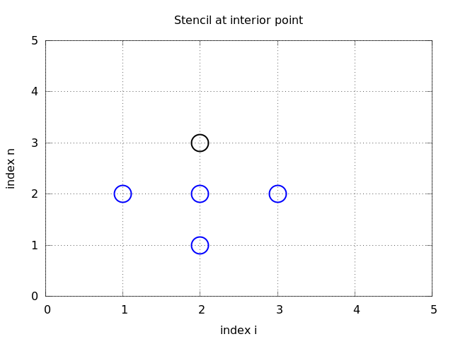
Mesh in space and time for a 1D wave equation

Fulfilling the equation at the mesh points

For a numerical solution by the finite difference method, we relax the condition that (1) holds at all points in the space-time domain \((0,L)\times (0,T]\) to the requirement that the PDE is fulfilled at the interior mesh points:

(6)\[ \frac{\partial^2}{\partial t^2} u(x_i, t_n) = c^2\frac{\partial^2}{\partial x^2} u(x_i, t_n),\]

for \(i=1,\ldots,N_x-1\) and \(n=1,\ldots,N_t-1\). For \(n=0\) we have the initial conditions \(u=I(x)\) and \(u_t=0\), and at the boundaries \(i=0,N_x\) we have the boundary condition \(u=0\).

Replacing derivatives by finite differences

The second-order derivatives can be replaced by central differences. The most widely used difference approximation of the second-order derivative is

\[\frac{\partial^2}{\partial t^2}u(x_i,t_n)\approx \frac{u_i^{n+1} - 2u_i^n + u^{n-1}_i}{\Delta t^2}{\thinspace .}\]

It is convenient to introduce the finite difference operator notation

\[[D_tD_t u]^n_i = \frac{u_i^{n+1} - 2u_i^n + u^{n-1}_i}{\Delta t^2}{\thinspace .} A similar approximation of the second-order derivative in the $x$ direction reads !bt \frac{\partial^2}{\partial x^2}u(x_i,t_n)\approx \frac{u_{i+1}^{n} - 2u_i^n + u^{n}_{i-1}}{\Delta x^2} = [D_xD_x u]^n_i {\thinspace .}\]

Algebraic version of the PDE

We can now replace the derivatives in (6) and get

(7)\[ \frac{u_i^{n+1} - 2u_i^n + u^{n-1}_i}{\Delta t^2} = c^2\frac{u_{i+1}^{n} - 2u_i^n + u^{n}_{i-1}}{\Delta x^2},\]

or written more compactly using the operator notation:

(8)\[ [D_tD_t u = c^2 D_xD_x]^{n}_i {\thinspace .}\]

Algebraic version of the initial conditions

We also need to replace the derivative in the initial condition (3) by a finite difference approximation. A centered difference of the type

\[\frac{\partial}{\partial t} u(x_i,t_n)\approx \frac{u^1_i - u^{-1}_i}{2\Delta t} = [D_{2t} u]^0_i,\]

seems appropriate. In operator notation the initial condition is written as

\[[D_{2t} u]^n_i = 0,\quad n=0 {\thinspace .}\]

Writing out this equation and ordering the terms give

(9)\[ u^{n-1}_i=u^{n+1}_i,\quad i=0,\ldots,N_x,\ n=0{\thinspace .}\]

The other initial condition can be computed by

\[u_i^0 = I(x_i),\quad i=0,\ldots,N_x{\thinspace .}\]

Formulating a recursive algorithm

We assume that \(u^n_i\) and \(u^{n-1}_i\) are already computed for \(i=0,\ldots,N_x\). The only unknown quantity in (7) is therefore \(u^{n+1}_i\), which we can solve for:

(10)\[ u^{n+1}_i = -u^{n-1}_i + 2u^n_i + C^2 \left(u^{n}_{i+1}-2u^{n}_{i} + u^{n}_{i-1}\right),\]

where we have introduced the parameter

\[C = c\frac{\Delta t}{\Delta x},\]

known as the (dimensionless) Courant number. We see that the discrete version of the PDE features only one parameter, \(C\), which is therefore the key parameter that governs the quality of the numerical solution. Both the primary physical parameter \(c\) and the numerical parameters \(\Delta x\) and \(\Delta t\) are lumped together in \(C\).

Given that \(u^{n-1}_i\) and \(u^n_i\) are computed for \(i=0,\ldots,N_x\), we find new values at the next time level by applying the formula (10) for \(i=1,\ldots,N_x-1\). Figure Mesh in space and time for a 1D wave equation illustrates the points that are used to compute \(u^3_2\). For the boundary points, \(i=0\) and \(i=N_x\), we apply the boundary conditions \(u_i^{n+1}=0\).

A problem with (10) arises when \(n=0\) since the formula for \(u^1_i\) involves \(u^{-1}_i\), which is an undefined quantity outside the time mesh (and the time domain). However, we can use the initial condition (9) in combination with (10) when \(n=0\) to arrive at a special formula for \(u_i^1\):

(11)\[ u_i^1 = u^0_i - \frac{1}{2} C^2\left(u^{n}_{i+1}-2u^{n}_{i} + u^{n}_{i-1}\right) {\thinspace .}\]

Figure Modified stencil for the first time step illustrates how (11) connects four instead of five points: \(u^1_2\), \(u_1^0\), \(u_2^0\), and \(u_3^0\).

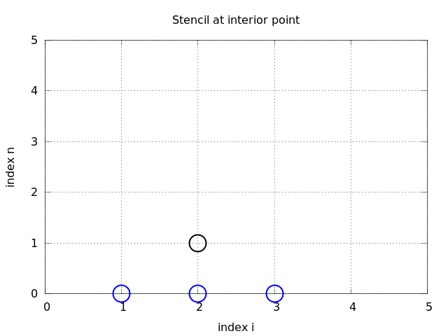
Modified stencil for the first time step

We can now summarize the computational algorithm:

1. Compute \(u^0_i=I(x_i)\) for \(i=0,\ldots,N_x\)
2. Compute \(u^1_i\) by (11) and set \(u_i^1=0\) for the boundary points \(i=0\) and \(i=N_x\), for \(n=1,2,\ldots,N-1\),
3. For each time level \(n=1,2,\ldots,N_t-1\)

1. apply (10) to find \(u^{n+1}_i\) for \(i=1,\ldots,N_x-1\)
2. set \(u^{n+1}_i=0\) for the boundary points \(i=0\), \(i=N_x\).

The algorithm essentially consists of moving a finite difference stencil through all the mesh points, which is illustrated by an animation in a web page or a movie file.

Sketch of an implementation

In a Python implementation of this algorithm, we use the array elements u[i] to store \(u^{n+1}_i\), u_1[i] to store \(u^n_i\), and u_2[i] to store \(u^{n-1}_i\). Our naming convention is use u for the unknown new spatial field to be computed, u_1 as the solution at one time step back in time, u_2 as the solution two time steps back in time and so forth.

The algorithm only needs to access the three most recent time levels, so we need only three arrays for \(u_i^{n+1}\), \(u_i^n\), and \(u_i^{n-1}\), \(i=0,\ldots,N_x\). Storing all the solutions in a two-dimensional array of size \((N_x+1)\times (N_t+1)\) would be possible in this simple one-dimensional PDE problem, but is normally out of the question in three-dimensional (3D) and large two-dimensional (2D) problems. We shall therefore in all our programs for solving PDEs have the unknown in memory at as few time levels as possible.

The following Python snippet realizes the steps in the computational algorithm.

# Given mesh points as arrays x and t (x[i], t[n])
dx = x[1] - x[0]
dt = t[1] - t[0]
C = c*dt/dx            # Courant number
Nt = len(t)-1
C2 = C**2              # Help variable in the scheme

# Set initial condition u(x,0) = I(x)
for i in range(0, Nx+1):
    u_1[i] = I(x[i])

# Apply special formula for first step, incorporating du/dt=0
for i in range(1, Nx):
    u[i] = u_1[i] - 0.5*C**2(u_1[i+1] - 2*u_1[i] + u_1[i-1])
u[0] = 0;  u[Nx] = 0   # Enforce boundary conditions

# Switch variables before next step
u_2[:], u_1[:] = u_1, u

for n in range(1, Nt):
    # Update all inner mesh points at time t[n+1]
    for i in range(1, Nx):
        u[i] = 2u_1[i] - u_2[i] - \
               C**2(u_1[i+1] - 2*u_1[i] + u_1[i-1])

    # Insert boundary conditions
    u[0] = 0;  u[Nx] = 0

    # Switch variables before next step
    u_2[:], u_1[:] = u_1, u

Verification (1)

Before implementing the algorithm, it is convenient to add a source term to the PDE (1) since it gives us more freedom in finding test problems for verification. In particular, the source term allows us to use manufactured solutions for software testing, where we simply choose some function as solution, fit the corresponding source term, and define boundary and initial conditions consistent with the chosen solution. Such solutions will seldom fulfill the initial condition (3) so we need to generalize this condition to \(u_t=V(x)\).

A slightly generalized model problem

We now address the following extended initial-boundary value problem for one-dimensional wave phenomena:

(12)\[ u_{tt} = c^2 u_{xx} + f(x,t), \quad x\in (0,L),\ t\in (0,T]\]

(13)\[ u(x,0) = I(x), \quad x\in [0,L]\]

(14)\[ u_t(x,0) = V(x), \quad x\in [0,L]\]

(15)\[\begin{split} u(0,t) = 0, \quad t>0\end{split}\]

(16)\[\begin{split} u(L,t) = 0, \quad t>0\end{split}\]

Sampling the PDE at \((x_i,t_n)\) and using the same finite difference approximations as above, yields

(17)\[ [D_tD_t u = c^2 D_xD_x + f]^{n}_i {\thinspace .}\]

Writing this out and solving for the unknown \(u^{n+1}_i\) results in

(18)\[ u^{n+1}_i = -u^{n-1}_i + 2u^n_i + C^2 (u^{n}_{i+1}-2u^{n}_{i} + u^{n}_{i-1}) + \Delta t^2 f^n_i\]\[ {\thinspace .}\]

The equation for the first time step must be rederived. The discretization of the initial condition \(u_t = V(x)\) at \(t=0\) becomes

\[[D_{2t}u = V]^0_i\quad\Rightarrow\quad u^{-1}_i = u^{1}_i - 2\Delta t V_i,\]

which, when inserted in (18) for \(n=0\), gives the special formula

(19)\[ u^{1}_i = u^0_i - \Delta t V_i + {\frac{1}{2}} C^2 \left(u^{n}_{i+1}-2u^{n}_{i} + u^{n}_{i-1}\right) + \frac{1}{2}\Delta t^2 f^n_i\]\[ {\thinspace .}\]

Using an analytical solution of physical significance

Many wave problems feature sinusoidal oscillations in time and space. For example, the original PDE problem (1)-(5) allows a solution

(20)\[ {u_{\small\mbox{e}}}(x,y,t)) = A\sin\left(\frac{\pi}{L}x\right) \cos\left(\frac{\pi}{L}ct\right){\thinspace .}\]

This \({u_{\small\mbox{e}}}\) fulfills the PDE with \(f=0\), boundary conditions \({u_{\small\mbox{e}}}(0,t)={u_{\small\mbox{e}}}(L,0)=0\), as well as initial conditions \(I(x)=A\sin\left(\frac{\pi}{L}x\right)\) and \(V=0\).

It is common to use such exact solutions of physical interest to verify implementations. However, the numerical solution \(u^n_i\) will only be an approximation to \({u_{\small\mbox{e}}}(x_i,t_n)\). We no have knowledge of the precise size of the error in this approximation, and therefore we can never know if discrepancies between the computed \(u^n_i\) and \({u_{\small\mbox{e}}}(x_i,t_n)\) are caused by mathematical approximations or programming errors. In particular, if a plot of the computed solution \(u^n_i\) and the exact one eq:ref:wave:pde2:test:ue looks similar, many are attempted to claim that the implementation works, but there can still be serious programming errors although color plots look nice.

The only way to use exact physical solutions like (20) for serious and thorough verification is to run a series of finer and finer meshes, measure the integrated error in each mesh, and from this information estimate the convergence rate. If these rates are very close to 2, we have strong evidence that the implementation works.

Manufactured solution

One problem with the exact solution (20) is that it requires a simplification (\(V=0, f=0\)) of the implemented problem (12)-(16). An advantage of using a manufactured solution is that we can test all terms in the PDE problem. The idea of this approach is to set up some chosen solution and fit the source term, boundary conditions, and initial conditions to be compatible with the chosen solution. Given that our boundary conditions in the implementation are \(u(0,t)=u(L,t)=0\), we must choose a solution that fulfills these conditions. One example is

\[{u_{\small\mbox{e}}}(x,t) = x(L-x)\sin t{\thinspace .}\]

Inserted in the PDE \(u_{tt}=c^2u_{xx}+f\) we get

\[-x(L-x)\sin t = -2\sin t + f\quad\Rightarrow f = (2 - x(L-x))\sin t{\thinspace .}\]

The initial conditions become

\[\begin{split}u(x,0) =& I(x) = 0,\\ u_t(x,0) &= V(x) = (2 - x(L-x))\cos t{\thinspace .}\end{split}\]

To verify the code, we run a series of refined meshes and compute the convergence rates. In more detail, we keep \(\Delta t/\Delta x\) constant for each mesh, implying that \(C\) is also constant throughout the experiments. A common discretization parameter \(h = \Delta t\) is introduced. For a given \(C\) (and \(c\)), \(\Delta x ch/C\). We choose an initial time cell size \(h_0\) and run experiments with decreasing \(h\): \(h_i=2^{-i}h_0\), \(i=1,2,\ldots,m\). Halving the cell size in each experiment is not necessary, but common. For each experiment we must record a scalar measure of the error. As will be shown later, it is expected that such error measures are proportional to \(h^2\). A standard choice of error measure is the \(\ell^2\) or \(\ell^\infty\) norm of the error mesh function \(e^n_i\):

\[||e^n_i||_{\ell^2} = \left( \Delta t\Delta x\sum_{n=0}^{N_t}\sum_{i=0}^{N_x} (e^n_i)^2\right)^{\frac{1}{2}},\quad e^n_i = {u_{\small\mbox{e}}}(x_i,t_n)-u^n_i,\]

\[||e^n_i||_{\ell^\infty} = \max_{i,n} |e^i_n|{\thinspace .}\]

In Python, one can compute \(\sum_{i}(e^{n+1}_i)^2\) at each time step and accumulate the value in some sum variable, say e2_sum. At the final time step one can do sqrt(dt*dx*e2_sum). For the \(\ell^\infty\) norm one must compare the maximum error at a time level (e.max()) with the global maximum over the time domain: e_max = max(e_max, e.max()).

An alternative error measure is to use a spatial norm at one time step only, e.g., the end time \(T\):

\[||e^n_i||_{\ell^2} = \left( \Delta x\sum_{i=0}^{N_x} (e^n_i)^2\right)^{\frac{1}{2}},\quad e^n_i = {u_{\small\mbox{e}}}(x_i,t_n)-u^n_i,\]

\[||e^n_i||_{\ell^\infty} = \max_{0\leq i\leq N_x} |e^i_{n}|{\thinspace .}\]

Let \(E_i\) be the error measure in experiment (mesh) number \(i\) and let \(h_i\) be the corresponding discretization parameter (\(h\)). We expect an error model \(E_i = Ch_i^r\), here with \(r=0\). To estimate \(r\), we can compare two consecutive experiments and compute

\[r_i = \frac{\ln E_{i+1}/E_{i}}{\ln h_{i+1}/h_{i}},\quad i=0,\ldots,m-1{\thinspace .}\]

We should observe that \(r_i\) approaches \(2\) as \(i\) increases.

The next section describes a method of manufactured solutions where do not need to compute error measures and check that they converge as expected as the mesh is refined.

Constructing an exact solution of the discrete equations

For verification purposes we shall use a solution that is quadratic in space and linear in time. More specifically, our choice of the manufactured solution is

(21)\[ {u_{\small\mbox{e}}} (x,t) = x(L-x)(1+{\frac{1}{2}}t),\]

which by insertion in the PDE leads to \(f(x,t)=2(1+t)c^2\). This \({u_{\small\mbox{e}}}\) fulfills the boundary conditions and is compatible with \(I(x)=x(L-x)\) and \(V(x)={\frac{1}{2}}x(L-x)\).

A key feature of the chosen \({u_{\small\mbox{e}}}\) is that it is also an exact solution of the discrete equations. To realize this very important result, we first establish the results

\[\lbrack D_tD_t t^2\rbrack^n = \frac{t_{n+1}^2 - 2t_n^2 + t_{n-1}^2}{\Delta t^2} = (n+1)^2 -n^2 + (n-1)^2 = 2,\]

\[\lbrack D_tD_t t\rbrack^n = \frac{t_{n+1} - 2t_n + t_{n-1}}{\Delta t^2} = \frac{((n+1) -n + (n-1))\Delta t}{\Delta t^2} = 0 {\thinspace .}\]

Hence,

\[[D_tD_t {u_{\small\mbox{e}}}]^n_i = x_i(L-x_i)[D_tD_t (1+{\frac{1}{2}}t)]^n = x_i(L-x_i){\frac{1}{2}}[D_tD_t t]^n = 0,\]

and

\[\begin{split}\lbrack D_xD_x {u_{\small\mbox{e}}}\rbrack^n_i &= (1+{\frac{1}{2}}t_n)\lbrack D_xD_x (xL-x^2)\rbrack_i = (1+{\frac{1}{2}}t_n)\lbrack LD_xD_x x - D_xD_x x^2\rbrack_i \\ &= -2(1+{\frac{1}{2}}t_n) {\thinspace .}\end{split}\]

Now, \(f^n_i = 2(1+{\frac{1}{2}}t_n)c^2\) and we get

\[[D_tD_t {u_{\small\mbox{e}}} - c^2D_xD_x{u_{\small\mbox{e}}} - f]^n_i = 0 - c^2(-1)2(1 + {\frac{1}{2}}t_n + 2(1+{\frac{1}{2}}t_n)c^2 = 0{\thinspace .}\]

Moreover, \({u_{\small\mbox{e}}}(x_i,0)=I(x_i)\), \(\partial {u_{\small\mbox{e}}}/\partial t = V(x_i)\) at \(t=0\), and \({u_{\small\mbox{e}}}(x_0,t)={u_{\small\mbox{e}}}(x_{N_x},0)=0\). Also the modified scheme for the first time step is fulfilled by \({u_{\small\mbox{e}}}(x_i,t_n)\).

Therefore, the exact solution \({u_{\small\mbox{e}}}(x,t)=x(L-x)(1+t/2)\) of the PDE problem is also an exact solution of the discrete problem. We can use this result to check that the computed \(u^n_i\) vales from an implementation equals \({u_{\small\mbox{e}}}(x_i,t_n)\) within machine precision, regardless of the mesh spacings \(\Delta x\) and \(\Delta t\)! Nevertheless, there might be stability restrictions on \(\Delta x\) and \(\Delta t\), so the test can only be run for a mesh that is compatible with the stability criterion (which in the present case is \(C\leq 1\), to be derived later).

Note

A product of quadratic or linear expressions in the various independent variables, as shown above, will often fulfill both the continuous and discrete PDE problem and can therefore be very useful solutions for verifying implementations. However, for 1D wave equations of the type \(u_t=c^2u_{xx}\) we shall see that there is always another much more powerful way of generating exact solutions (just set \(C=1\)).