Generalization: reflecting boundaries

The boundary condition \(u=0\) makes \(u\) change sign at the boundary, while the condition \(u_x=0\) perfectly reflects the wave, see a web page or a movie file for demonstration. Our next task is to explain how to implement the boundary condition \(u_x=0\), which is more complicated to express numerically and also to implement than a given value of \(u\). We shall present two methods for implementing \(u_x=0\) in a finite difference scheme, one based on deriving a modified stencil at the boundary, and another one based on extending the mesh with ghost cells and ghost points.

Neumann boundary condition

When a wave hits a boundary and is to be reflected back, one applies the condition

(1)\[ \frac{\partial u}{\partial n} \equiv \boldsymbol{n}\cdot\nabla u = 0\]\[ {\thinspace .}\]

The derivative \(\partial /\partial n\) is in the outward normal direction from a general boundary. For a 1D domain \([0,L]\), we have that

\[\left.\frac{\partial}{\partial n}\right\vert_{x=L} = \frac{\partial}{\partial x},\quad \left.\frac{\partial}{\partial n}\right\vert_{x=0} = - \frac{\partial}{\partial x}{\thinspace .}\]

Boundary condition terminology

Boundary conditions that specify the value of \(\partial u/\partial n\), or shorter \(u_n\), are known as Neumann conditions, while Dirichlet conditions refer to specifications of \(u\). When the values are zero (\(\partial u/\partial n=0\) or \(u=0\)) we speak about homogeneous Neumann or Dirichlet conditions.

Discretization of derivatives at the boundary

How can we incorporate the condition (1) in the finite difference scheme? Since we have used central differences in all the other approximations to derivatives in the scheme, it is tempting to implement (1) at \(x=0\) and \(t=t_n\) by the difference

(2)\[ \frac{u_{-1}^n - u_1^n}{2\Delta x} = 0 {\thinspace .}\]

The problem is that \(u_{-1}^n\) is not a \(u\) value that is being computed since the point is outside the mesh. However, if we combine (2) with the scheme .. (2.10)

for \(i=0\),

(3)\[ u^{n+1}_i = -u^{n-1}_i + 2u^n_i + C^2 \left(u^{n}_{i+1}-2u^{n}_{i} + u^{n}_{i-1}\right),\]

we can eliminate the fictitious value \(u_{-1}^n\). We see that \(u_{-1}^n=u_1^n\) from (2), which can be used in (3) to arrive at a modified scheme for the boundary point \(u_0^{n+1}\):

\[u^{n+1}_i = -u^{n-1}_i + 2u^n_i + 2C^2 \left(u^{n}_{i+1}-u^{n}_{i}\right),\quad i=0 {\thinspace .}\]

Figure Modified stencil at a boundary with a Neumann condition visualizes this equation for computing \(u^3_0\) in terms of \(u^2_0\), \(u^1_0\), and \(u^2_1\).

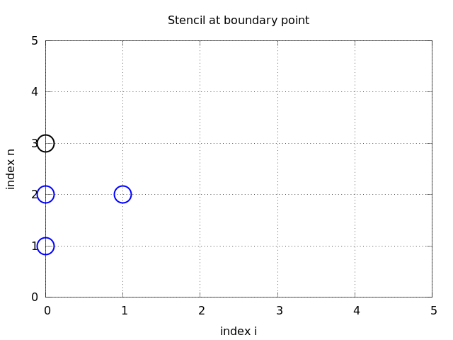
Modified stencil at a boundary with a Neumann condition

Similarly, (1) applied at \(x=L\) is discretized by a central difference

(4)\[ \frac{u_{N_x+1}^n - u_{N_x-1}^n}{2\Delta x} = 0 {\thinspace .}\]

Combined with the scheme for \(i=N_x\) we get a modified scheme for the boundary value \(u_{N_x}^{n+1}\):

\[u^{n+1}_i = -u^{n-1}_i + 2u^n_i + 2C^2 \left(u^{n}_{i-1}-u^{n}_{i}\right),\quad i=N_x {\thinspace .}\]

The modification of the scheme at the boundary is also required for the special formula for the first time step. How the stencil moves through the mesh and is modified at the boundary can be illustrated by an animation in a web page or a movie file.

Implementation of Neumann conditions

The implementation of the special formulas for the boundary points can benefit from using the general formula for the interior points also at the boundaries, but replacing \(u_{i-1}^n\) by \(u_{i+1}^n\) when computing \(u_i^{n+1}\) for \(i=0\) and \(u_{i+1}^n\) by \(u_{i-1}^n\) for \(i=N_x\). This is achieved by just replacing the index \(i-1\) by \(i+1\) for \(i=0\) and \(i+1\) by \(i-1\) for \(i=N_x\). In a program, we introduce variables to hold the value of the offset indices: im1 for i-1 and ip1 for i+1. It is now just a manner of defining im1 and ip1 properly for the internal points and the boundary points. The coding for the latter reads

i = 0
ip1 = i+1
im1 = ip1  # i-1 -> i+1
u[i] = u_1[i] + C2*(u_1[im1] - 2*u_1[i] + u_1[ip1])

i = Nx
im1 = i-1
ip1 = im1  # i+1 -> i-1
u[i] = u_1[i] + C2*(u_1[im1] - 2*u_1[i] + u_1[ip1])

We can in fact create one loop over both the internal and boundary points and use only one updating formula:

for i in range(0, Nx+1):
    ip1 = i+1 if i < Nx else i-1
    im1 = i-1 if i > 0  else i+1
    u[i] = u_1[i] + C2*(u_1[im1] - 2*u_1[i] + u_1[ip1])

The program wave1D_dn0.py contains a complete implementation of the 1D wave equation with boundary conditions \(u_x = 0\) at \(x=0\) and \(x=L\).

Index set notation

We shall introduce a special notation for index sets, consisting of writing \(x_i\), \(i\in{\mathcal{I}_x}\), instead of \(i=0,\ldots,N_x\). Obviously, \({\mathcal{I}_x}\) must be the set \({\mathcal{I}_x} =\{0,\ldots,N_x\}\), but it is often advantageous to have a symbol for this set rather than specifying all its elements. This saves writing and makes specification of algorithms and implementation of computer code easier.

The first index in the set will be denoted \({{\mathcal{I^0}_x}}\) and the last \({\mathcal{I^{-1}_x}}\). Sometimes we need to count from the second element in the set, and the notation \({{\mathcal{I^+}_x}}\) is then used. Correspondingly, \({{\mathcal{I^-}_x}}\) means \(\{0,\ldots,N_x-1\}\). All the indices corresponding to inner grid points are \({{\mathcal{I^i}_x}}=\{1,\ldots,N_x-1\}\). For the time domain we find it natural to explicitly use 0 as the first index, so we will usually write \(n=0\) and \(t_0\) rather than \(n={\mathcal{I}_t}^0\). We also avoid notation like \(x_{{\mathcal{I^{-1}_x}}}\) and will instead use \(x_i\), \(i={\mathcal{I^{-1}_x}}\).

The Python code associated with index sets applies the following conventions:

An important feature of the index set notation is that it keeps our formulas and code independent of how we count mesh points. For example, the notation \(i\in{\mathcal{I}_x}\) or \(i={{\mathcal{I^0}_x}}\) remains the same whether \({\mathcal{I}_x}\) is defined as above or as starting at 1, i.e., \({\mathcal{I}_x}=\{1,\ldots,Q\}\). Similarly, we can in the code define Ix=range(Nx+1) or Ix=range(1,Q), and expressions like Ix[0] and Ix[1:-1] remain correct. One application where the index set notation is convenient is conversion of code from a language where arrays has base index 0 (e.g., Python and C) to languages where the base index is 1 (e.g., MATLAB and Fortran). Another important application is implementation of Neumann conditions via ghost points (see next section).

For the current problem setting in the \(x,t\) plane, we work with the index sets

\[{\mathcal{I}_x} = \{0,\ldots,N_x\},\quad {\mathcal{I}_t} = \{0,\ldots,N_t\},\]

defined in Python as

Ix = range(0, Nx+1)
It = range(0, Nt+1)

A finite difference scheme can with the index set notation be specified as

\[\begin{split}u^{n+1}_i &= -u^{n-1}_i + 2u^n_i + C^2 \left(u^{n}_{i+1}-2u^{n}_{i}+u^{n}_{i-1}\right), \quad i\in{{\mathcal{I^i}_x}},\ n\in{{\mathcal{I^i}_t}},\\ u_i &= 0, \quad i={{\mathcal{I^0}_x}},\ n\in{{\mathcal{I^i}_t}},\\ u_i &= 0, \quad i={\mathcal{I^{-1}_x}},\ n\in{{\mathcal{I^i}_t}},\end{split}\]

and implemented by code like

for n in It[1:-1]:
    for i in Ix[1:-1]:
        u[i] = - u_2[i] + 2*u_1[i] + \
               C2*(u_1[i-1] - 2*u_1[i] + u_1[i+1])
    i = Ix[0];  u[i] = 0
    i = Ix[-1]; u[i] = 0

Note

The program wave1D_dn.py applies the index set notation and solves the 1D wave equation \(u_{tt}=c^2u_{xx}+f(x,t)\) with quite general boundary and initial conditions:

• \(x=0\): \(u=U_0(t)\) or \(u_x=0\)
• \(x=L\): \(u=U_L(t)\) or \(u_x=0\)
• \(t=0\): \(u=I(x)\)
• \(t=0\): \(u_t=I(x)\)

The program combines Dirichlet and Neumann conditions, scalar and vectorized implementation of schemes, and the index notation into one piece of code. A lot of test examples are also included in the program:

• A rectangular plug profile as initial condition (easy to use as test example as the rectangle should jump one cell per time step when \(C=1\), without any numerical errors).
• A Gaussian function as initial condition.
• A triangular profile as initial condition, which resembles the typical initial shape of a guitar string.
• A sinusoidal variation of \(u\) at \(x=0\) and either \(u=0\) or \(u_x=0\) at \(x=L\).
• An exact analytical solution \(u(x,t)=\cos(m\pi t/L)\sin({\frac{1}{2}}m\pi x/L)\), which can be used for convergence rate tests.

Alternative implementation via ghost cells

Idea

Instead of modifying the scheme at the boundary, we can introduce extra points outside the domain such that the fictitious values \(u_{-1}^n\) and \(u_{N_x+1}^n\) are defined in the mesh. Adding the intervals \([-\Delta x,0]\) and \([L, L+\Delta x]\), often referred to as ghost cells, to the mesh gives us all the needed mesh points, corresponding to \(i=-1,0,\ldots,N_x,N_x+1\). The extra points \(i=-1\) and \(i=N_x+1\) are known as ghost points, and values at these points, \(u_{-1}^n\) and \(u_{N_x+1}^n\), are called ghost values.

The important idea is to ensure that we always have

\[u_{-1}^n = u_{1}^n\hbox{ and } u_{N_x+1}^n = u_{N_x-1}^n,\]

because then the application of the standard scheme at a boundary point \(i=0\) or \(i=N_x\) will be correct and guarantee that the solution is compatible with the boundary condition \(u_x=0\).

Implementation (2)

The u array now needs extra elements corresponding to the ghost cells and points. Two new point values are needed:

u   = zeros(Nx+3)

The arrays u_1 and u_2 must be defined accordingly.

Unfortunately, a major indexing problem arises with ghost cells. The reason is that Python indices must start at 0 and u[-1] will always mean the last element in u. This fact gives, apparently, a mismatch between the mathematical indices \(i=-1,0,\ldots,N_x+1\) and the Python indices running over u: 0,..,Nx+2. One remedy is to change the mathematical notation of the scheme, as in

\[u^{n+1}_i = \cdots,\quad i=1,\ldots,N_x+1,\]

meaning that the ghost points correspond to \(i=0\) and \(i=N_x+1\). A better solution is to use the ideas of the section Index set notation: we hide the specific index value in an index set and operate with inner and boundary points using the index set notation.

To this end, we define u with proper length and Ix to be the corresponding indices for the real physical points:

u = zeros(Nx+3)
Ix = range(1, u.shape[0]-1)

That is, the boundary points have indices Ix[0] and Ix[-1] (as before). We first update the solution at all physical mesh points (i.e., interior points in the mesh extended with ghost cells):

for i in Ix:
    u[i] = - u_2[i] + 2*u_1[i] + \
           C2*(u_1[i-1] - 2*u_1[i] + u_1[i+1])

It remains to update the ghost points. For a boundary condition \(u_x=0\), the ghost value must equal to the value at the associated inner mesh point. Computer code makes this statement precise:

i = Ix[0]          # x=0 boundary
u[i-1] = u[i+1]
i = Ix[-1]         # x=L boundary
u[i+1] = u[i-1]

The physical solution to be plotted is now in u[1:-1], so this slice is the quantity to be returned from a solver function. A complete implementation appears in the program wave1D_dn0_ghost.py.

Warning

We have to be careful with how the spatial and temporal mesh points are stored. Say we let x be the physical mesh points,

x = linspace(0, L, Nx+1)

“Standard coding” of the initial condition,

for i in Ix:
    u_1[i] = I(x[i])

becomes wrong, since u_1 and x have different lengths and the index i corresponds to two different mesh points. In fact, x[i] corresponds to u[1+i]. A correct implementation is

for i in Ix:
    u_1[i] = I(x[i-Ix[0]])

Similarly, a source term usually coded as f(x[i], t[n]) is incorrect if x is defined to be the physical points.

An alternative remedy is to let x also cover the ghost points such that u[i] is the value at x[i]. This is the recommended approach.

The ghost cell is only added to the boundary where we have a Neumann condition. Suppose we have a Dirichlet condition at \(x=L\) and a homogeneous Neumann condition at \(x=0\). The relevant implementation then becomes

u = zeros(Nx+2)
Ix = range(0, u.shape[0]-1)
...
for i in Ix[:-1]:
    u[i] = - u_2[i] + 2*u_1[i] + \
           C2*(u_1[i-1] - 2*u_1[i] + u_1[i+1]) + \
           dt2*f(x[i], t[n])
i = Ix[-1]
u[i] = U_0       # set Dirichlet value
i = Ix[0]
u[i+1] = u[i-1]  # update ghost value

The physical solution to be plotted is now in u[1:].

Generalization: variable wave velocity

Our next generalization of the 1D wave equation (2.1) or (2.12) is to allow for a variable wave velocity \(c\): \(c=c(x)\), usually motivated by wave motion in a domain composed of different physical media with different properties for propagating waves and hence different wave velocities \(c\). Figure

Left: wave entering another medium; right: transmitted and reflected wave

The model PDE with a variable coefficient

Instead of working with the squared quantity \(c^2(x)\) we shall for notational convenience introduce \(q(x) = c^2(x)\). A 1D wave equation with variable wave velocity often takes the form

(5)\[ \frac{\partial^2 u}{\partial t^2} = \frac{\partial}{\partial x}\left( q(x) \frac{\partial u}{\partial x}\right) + f(x,t)\]\[ {\thinspace .}\]

This equation sampled at a mesh point \((x_i,t_n)\) reads

\[\frac{\partial^2 }{\partial t^2} u(x_i,t_n) = \frac{\partial}{\partial x}\left( q(x_i) \frac{\partial}{\partial x} u(x_i,t_n)\right) + f(x_i,t_n),\]

where the only new term is

\[\frac{\partial}{\partial x}\left( q(x_i) \frac{\partial}{\partial x} u(x_i,t_n)\right) = \left[ \frac{\partial}{\partial x}\left( q(x) \frac{\partial u}{\partial x}\right)\right]^n_i {\thinspace .}\]

Discretizing the variable coefficient

The principal idea is to first discretize the outer derivative. Define

\[\phi = q(x) \frac{\partial u}{\partial x},\]

and use a centered derivative around \(x=x_i\) for the derivative of \(\phi\):

\[\left[\frac{\partial\phi}{\partial x}\right]^n_i \approx \frac{\phi_{i+\frac{1}{2}} - \phi_{i-\frac{1}{2}}}{\Delta x} = [D_x\phi]^n_i {\thinspace .}\]

Then discretize

\[\phi_{i+\frac{1}{2}} = q_{i+\frac{1}{2}} \left[\frac{\partial u}{\partial x}\right]^n_{i+\frac{1}{2}} \approx q_{i+\frac{1}{2}} \frac{u^n_{i+1} - u^n_{i}}{\Delta x} = [q D_x u]_{i+\frac{1}{2}}^n {\thinspace .}\]

Similarly,

\[\phi_{i-\frac{1}{2}} = q_{i-\frac{1}{2}} \left[\frac{\partial u}{\partial x}\right]^n_{i-\frac{1}{2}} \approx q_{i-\frac{1}{2}} \frac{u^n_{i} - u^n_{i-1}}{\Delta x} = [q D_x u]_{i-\frac{1}{2}}^n {\thinspace .}\]

These intermediate results are now combined to

(6)\[ \left[ \frac{\partial}{\partial x}\left( q(x) \frac{\partial u}{\partial x}\right)\right]^n_i \approx \frac{1}{\Delta x^2} \left( q_{i+\frac{1}{2}} \left({u^n_{i+1} - u^n_{i}}\right) - q_{i-\frac{1}{2}} \left({u^n_{i} - u^n_{i-1}}\right)\right)\]\[ {\thinspace .}\]

With operator notation we can write the discretization as

(7)\[ \left[ \frac{\partial}{\partial x}\left( q(x) \frac{\partial u}{\partial x}\right)\right]^n_i \approx [D_xq D_x u]^n_i\]\[ {\thinspace .}\]

Remark

Many are tempted to use the chain rule on the term \(\frac{\partial}{\partial x}\left( q(x) \frac{\partial u}{\partial x}\right)\), but this is not a good idea when discretizing such a term.

Computing the coefficient between mesh points

If \(q\) is a known function of \(x\), we can easily evaluate \(q_{i+\frac{1}{2}}\) simply as \(q(x_{i+\frac{1}{2}})\) with \(x_{i+\frac{1}{2}} = x_i + \frac{1}{2}\Delta x\). However, in many cases \(c\), and hence \(q\), is only known as a discrete function, often at the mesh points \(x_i\). Evaluating \(q\) between two mesh points \(x_i\) and \(x_{i+1}\) can then be done by averaging in three ways:

(8)\[ q_{i+\frac{1}{2}} \approx \frac{1}{2}\left( q_{i} + q_{i+1}\right) = [\overline{q}^{x}]_i, \quad \hbox{(arithmetic mean)}\]

(9)\[ q_{i+\frac{1}{2}} \approx 2\left( \frac{1}{q_{i}} + \frac{1}{q_{i+1}}\right)^{-1}, \quad \hbox{(harmonic mean)}\]

(10)\[ q_{i+\frac{1}{2}} \approx \left(q_{i}q_{i+1}\right)^{1/2}, \quad \hbox{(geometric mean)}\]

The arithmetic mean in (8) is by far the most commonly used averaging technique.

With the operator notation from (8) we can specify the discretization of the complete variable-coefficient wave equation in a compact way:

(11)\[ \lbrack D_tD_t u = D_x\overline{q}^{x}D_x u + f\rbrack^{n}_i {\thinspace .}\]

From this notation we immediately see what kind of differences that each term is approximated with. The notation \(\overline{q}^{x}\) also specifies that the variable coefficient is approximated by an arithmetic mean, the definition being \([\overline{q}^{x}]_{i+\frac{1}{2}}=(q_i+q_{i+1})/2\). With the notation \([D_xq D_x u]^n_i\), we specify that \(q\) is evaluated directly, as a function, between the mesh points: \(q(x_{i-\frac{1}{2}})\) and \(q(x_{i+\frac{1}{2}})\).

Before any implementation, it remains to solve (11) with respect to \(u_i^{n+1}\):

\[u^{n+1}_i = - u_i^{n-1} + 2u_i^n + \nonumber\]

\[\quad \left(\frac{\Delta x}{\Delta t}\right)^2 \left( \frac{1}{2}(q_{i} + q_{i+1})(u_{i+1}^n - u_{i}^n) - \frac{1}{2}(q_{i} + q_{i-1})(u_{i}^n - u_{i-1}^n)\right) + \nonumber\]

(12)\[ \quad \Delta t^2 f^n_i {\thinspace .}\]

How a variable coefficient affects the stability

The stability criterion derived in the section Stability reads \(\Delta t\leq \Delta x/c\). If \(c=c(x)\), the criterion will depend on the spatial location. We must therefore choose a \(\Delta t\) that is small enough such that no mesh cell has \(\Delta x/c(x) >\Delta t\). That is, we must use the largest \(c\) value in the criterion:

\[\Delta t \leq \beta \frac{\Delta x}{\max_{x\in [0,L]}c(x)} {\thinspace .}\]

The parameter \(\beta\) is included as a safety factor: in some problems with a significantly varying \(c\) it turns out that one must choose \(\beta <1\) to have stable solutions (\(\beta =0.9\) may act as an all-round value).

Neumann condition and a variable coefficient

Consider a Neumann condition \(\partial u/\partial x=0\) at \(x=L=N_x\Delta x\), discretized as

\[\frac{u_{i+1}^{n} - u_{i-1}^n}{2\Delta x} = 0\quad u_{i+1}^n = u_{i-1}^n,\]

for \(i=N_x\). Using the scheme (12) at the end point \(i=N_x\) with \(u_{i+1}^n=u_{i-1}^n\) results in

\[u^{n+1}_i = - u_i^{n-1} + 2u_i^n + \nonumber\]

\[\quad \left(\frac{\Delta x}{\Delta t}\right)^2 \left( q_{i+\frac{1}{2}}(u_{i-1}^n - u_{i}^n) - q_{i-\frac{1}{2}}(u_{i}^n - u_{i-1}^n)\right) + \nonumber\]

\[\quad \Delta t^2 f^n_i\]

\[= - u_i^{n-1} + 2u_i^n + \left(\frac{\Delta x}{\Delta t}\right)^2 (q_{i+\frac{1}{2}} + q_{i-\frac{1}{2}})(u_{i-1}^n - u_{i}^n) + \Delta t^2 f^n_i\]

(13)\[ \approx - u_i^{n-1} + 2u_i^n + \left(\frac{\Delta x}{\Delta t}\right)^2 2q_{i}(u_{i-1}^n - u_{i}^n) + \Delta t^2 f^n_i {\thinspace .}\]

Here we used the approximation

\[q_{i+\frac{1}{2}} + q_{i-\frac{1}{2}} = q_i + \left(\frac{dq}{dx}\right)_i \Delta x + \left(\frac{d^2q}{dx^2}\right)_i \Delta x^2 + \cdots +\nonumber\]

\[\quad q_i - \left(\frac{dq}{dx}\right)_i \Delta x + \left(\frac{d^2q}{dx^2}\right)_i \Delta x^2 + \cdots\nonumber\]

\[= 2q_i + 2\left(\frac{d^2q}{dx^2}\right)_i \Delta x^2 + {\cal O}(\Delta x^4) \nonumber\]

\[\approx 2q_i {\thinspace .}\]

An alternative derivation may apply the arithmetic mean of \(q\) in (12), leading to the term

\[(q_i + \frac{1}{2}(q_{i+1}+q_{i-1}))(u_{i-1}^n-u_i^n){\thinspace .}\]

Since \(\frac{1}{2}(q_{i+1}+q_{i-1}) = q_i + {\cal O}(\Delta x^2)\), we end up with \(2q_i(u_{i-1}^n-u_i^n)\) for \(i=N_x\) as we did above.

A common technique in implementations of \(\partial u/\partial x=0\) boundary conditions is to assume \(dq/dx=0\) as well. This implies \(q_{i+1}=q_{i-1}\) and \(q_{i+1/2}=q_{i-1/2}\) for \(i=N_x\). The implications for the scheme are

\[u^{n+1}_i = - u_i^{n-1} + 2u_i^n + \nonumber\]

\[\quad \left(\frac{\Delta x}{\Delta t}\right)^2 \left( q_{i+\frac{1}{2}}(u_{i-1}^n - u_{i}^n) - q_{i-\frac{1}{2}}(u_{i}^n - u_{i-1}^n)\right) + \nonumber\]

\[\quad \Delta t^2 f^n_i\]

(14)\[ = - u_i^{n-1} + 2u_i^n + \left(\frac{\Delta x}{\Delta t}\right)^2 2q_{i-\frac{1}{2}}(u_{i-1}^n - u_{i}^n) + \Delta t^2 f^n_i {\thinspace .}\]

Implementation of variable coefficients

The implementation of the scheme with a variable wave velocity may assume that \(c\) is available as an array c[i] at the spatial mesh points. The following loop is a straightforward implementation of the scheme (12):

for i in range(1, Nx):
    u[i] = - u_2[i] + 2*u_1[i] + \
           C2*(0.5*(q[i] + q[i+1])*(u_1[i+1] - u_1[i])  - \
               0.5*(q[i] + q[i-1])*(u_1[i] - u_1[i-1])) + \
           dt2*f(x[i], t[n])

The coefficient C2 is now defined as (dt/dx)**2 and not as the squared Courant number since the wave velocity is variable and appears inside the parenthesis.

With Neumann conditions \(u_x=0\) at the boundary, we need to combine this scheme with the discrete version of the boundary condition, as shown in the section Neumann condition and a variable coefficient. Nevertheless, it would be convenient to reuse the formula for the interior points and just modify the indices ip1=i+1 and im1=i-1 as we did in the section Implementation of Neumann conditions. Assuming \(dq/dx=0\) at the boundaries, we can implement the scheme at the boundary with the following code.

i = 0
ip1 = i+1
im1 = ip1
u[i] = - u_2[i] + 2*u_1[i] + \
       C2*(0.5*(q[i] + q[ip1])*(u_1[ip1] - u_1[i])  - \
           0.5*(q[i] + q[im1])*(u_1[i] - u_1[im1])) + \
       dt2*f(x[i], t[n])

With ghost cells we can just reuse the formula for the interior points also at the boundary, provided that the ghost values of both \(u\) and \(q\) are correctly updated to ensure \(u_x=0\) and \(q_x=0\).

A vectorized version of the scheme with a variable coefficient at internal points in the mesh becomes

u[1:-1] = - u_2[1:-1] + 2*u_1[1:-1] + \
          C2*(0.5*(q[1:-1] + q[2:])*(u_1[2:] - u_1[1:-1]) -
              0.5*(q[1:-1] + q[:-2])*(u_1[1:-1] - u_1[:-2])) + \
          dt2*f(x[1:-1], t[n])

A more general model PDE with variable coefficients

Sometimes a wave PDE has a variable coefficient also in front of the time-derivative term:

(15)\[ \varrho(x)\frac{\partial^2 u}{\partial t^2} = \frac{\partial}{\partial x}\left( q(x) \frac{\partial u}{\partial x}\right) + f(x,t)\]\[ {\thinspace .}\]

A natural scheme is

\[[\varrho D_tD_t u = D_x\overline{q}^xD_x u + f]^n_i {\thinspace .}\]

We realize that the \(\varrho\) coefficient poses no particular difficulty because the only value \(\varrho_i^n\) enters the formula above (when written out). There is hence no need for any averaging of \(\varrho\). Often, \(\varrho\) will be moved to the right-hand side, also without any difficulty:

\[[D_tD_t u = \varrho^{-1}D_x\overline{q}^xD_x u + f]^n_i {\thinspace .}\]

Generalization: damping

Waves die out by two mechanisms. In 2D and 3D the energy of the wave spreads out in space, and energy conservation then requires the amplitude to decrease. This effect is not present in 1D. Damping is another cause of amplitude reduction. For example, the vibrations of a string die out because of damping due to air resistance and non-elastic effects in the string.

The simplest way of including damping is to add a first-order derivative to the equation (in the same way as friction forces enter a vibrating mechanical system):

(16)\[ \frac{\partial^2 u}{\partial t^2} + b\frac{\partial u}{\partial t} = c^2\frac{\partial^2 u}{\partial x^2} + f(x,t),\]

where \(b \geq 0\) is a prescribed damping coefficient.

A typical discretization of (16) in terms of centered differences reads

(17)\[ [D_tD_t u + bD_{2t}u = c^2D_xD_x u + f]^n_i {\thinspace .}\]

Writing out the equation and solving for the unknown \(u^{n+1}_i\) gives the scheme

(18)\[ u^{n+1}_i = (1 + {\frac{1}{2}}b\Delta t)^{-1}(({\frac{1}{2}}b\Delta t -1) u^{n-1}_i + 2u^n_i + C^2 \left(u^{n}_{i+1}-2u^{n}_{i} + u^{n}_{i-1}\right) + \Delta t^2 f^n_i),\]

for \(i\in{{\mathcal{I^i}_x}}\) and \(n\geq 1\). New equations must be derived for \(u^1_i\), and for boundary points in case of Neumann conditions.

The damping is very small in many wave phenomena and then only evident for very long time simulations. This makes the standard wave equation without damping relevant for a lot of applications.

Building a general 1D wave equation solver

The program wave1D_dn_vc.py is a fairly general code for 1D wave propagation problems that targets the following initial-boundary value problem

(19)\[ u_t = (c^2(x)u_x)_x + f(x,t),\quad x\in (0,L),\ t\in (0,T]\]

\[u(x,0) = I(x),\quad x\in [0,L]\]

\[u_t(x,0) = V(t),\quad x\in [0,L]\]

\[u(0,t) = U_0(t)\hbox{ or } u_x(0,t)=0,\quad t\in (0,T]\]

(20)\[ u(L,t) = U_L(t)\hbox{ or } u_x(L,t)=0,\quad t\in (0,T]\]

The solver function is a natural extension of the simplest solver function in the initial wave1D_u0_s.py program, extended with Neumann boundary conditions (\(u_x=0\)), a possibly time-varying boundary condition on \(u\) (\(U_0(t)\), \(U_L(t)\)), and a variable wave velocity. The different code segments needed to make these extensions are shown and commented upon in the preceding text.

The vectorization is only applied inside the time loop, not for the initial condition or the first time steps, since this initial work is negligible for long time simulations in 1D problems.

The following sections explain various more advanced programming techniques applied in the general 1D wave equation solver.

User action function as a class

A useful feature in the wave1D_dn_vc.py program is the specification of the user_action function as a class. Although the plot_u function in the viz function of previous wave1D*.py programs remembers the local variables in the viz function, it is a cleaner solution to store the needed variables together with the function, which is exactly what a class offers.

A class for flexible plotting, cleaning up files, and making a movie files like function viz and plot_u did can be coded as follows:

class PlotSolution:
    """
    Class for the user_action function in solver.
    Visualizes the solution only.
    """
    def __init__(self,
                 casename='tmp',    # Prefix in filenames
                 umin=-1, umax=1,   # Fixed range of y axis
                 pause_between_frames=None,  # Movie speed
                 backend='matplotlib',       # or 'gnuplot'
                 screen_movie=True, # Show movie on screen?
                 title='',          # Extra message in title
                 every_frame=1):    # Show every_frame frame
        self.casename = casename
        self.yaxis = [umin, umax]
        self.pause = pause_between_frames
        module = 'scitools.easyviz.' + backend + '_'
        exec('import %s as plt' % module)
        self.plt = plt
        self.screen_movie = screen_movie
        self.title = title
        self.every_frame = every_frame

        # Clean up old movie frames
        for filename in glob('frame_*.png'):
            os.remove(filename)

    def __call__(self, u, x, t, n):
        if n % self.every_frame != 0:
            return
        title = 't=%f' % t[n]
        if self.title:
            title = self.title + ' ' + title
        self.plt.plot(x, u, 'r-',
                     xlabel='x', ylabel='u',
                     axis=[x[0], x[-1],
                           self.yaxis[0], self.yaxis[1]],
                     title=title,
                     show=self.screen_movie)
        # pause
        if t[n] == 0:
            time.sleep(2)  # let initial condition stay 2 s
        else:
            if self.pause is None:
                pause = 0.2 if u.size < 100 else 0
            time.sleep(pause)

        self.plt.savefig('%s_frame_%04d.png' % (self.casename, n))

Understanding this class requires quite some familiarity with Python in general and class programming in particular.

The constructor shows how we can flexibly import the plotting engine as (typically) scitools.easyviz.gnuplot_ or scitools.easyviz.matplotlib_ (note the trailing underscore). With the screen_movie parameter we can suppress displaying each movie frame on the screen. Alternatively, for slow movies associated with fine meshes, one can set every_frame to, e.g., 10, causing every 10 frames to be shown.

The __call__ method makes PlotSolution instances behave like functions, so we can just pass an instance, say p, as the user_action argument in the solver function, and any call to user_action will be a call to p.__call__.

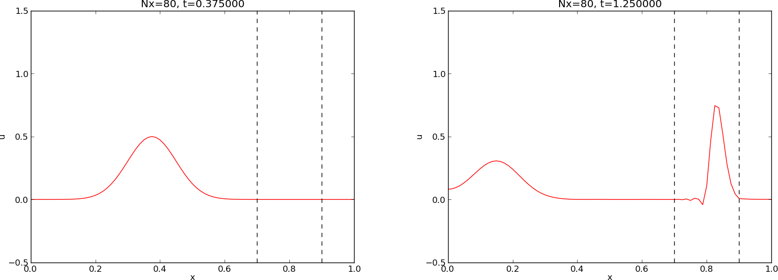
Pulse propagation in two media

The function pulse in wave1D_dn_vc.py demonstrates wave motion in heterogeneous media where \(c\) varies. One can specify an interval where the wave velocity is decreased by a factor slowness_factor (or increased by making this factor less than one). Four types of initial conditions are available: a rectangular pulse (plug), a Gaussian function (gaussian), a “cosine hat” consisting of one period of the cosine function (cosinehat), and half a period of a “cosine hat” (half-cosinehat). These peak-shaped initial conditions can be placed in the middle (loc='center') or at the left end (loc='left') of the domain. The pulse function is a flexible tool for playing around with various wave shapes and location of a medium with a different wave velocity:

def pulse(C=1, Nx=200, animate=True, version='vectorized', T=2,
          loc='center', pulse_tp='gaussian', slowness_factor=2,
          medium=[0.7, 0.9], every_frame=1, sigma=0.05):
    """
    Various peaked-shaped initial conditions on [0,1].
    Wave velocity is decreased by the slowness_factor inside
    medium. The loc parameter can be 'center' or 'left',
    depending on where the initial pulse is to be located.
    The sigma parameter governs the width of the pulse.
    """
    # Use scaled parameters: L=1 for domain length, c_0=1
    # for wave velocity outside the domain.
    L = 1.0
    c_0 = 1.0
    if loc == 'center':
        xc = L/2
    elif loc == 'left':
        xc = 0

    if pulse_tp in ('gaussian','Gaussian'):
        def I(x):
            return exp(-0.5*((x-xc)/sigma)**2)
    elif pulse_tp == 'plug':
        def I(x):
            return 0 if abs(x-xc) > sigma else 1
    elif pulse_tp == 'cosinehat':
        def I(x):
            # One period of a cosine
            w = 2
            a = w*sigma
            return 0.5*(1 + cos(pi*(x-xc)/a)) \
                   if xc - a <= x <= xc + a else 0

    elif pulse_tp == 'half-cosinehat':
        def I(x):
            # Half a period of a cosine
            w = 4
            a = w*sigma
            return cos(pi*(x-xc)/a) \
                   if xc - 0.5*a <= x <= xc + 0.5*a else 0
    else:
        raise ValueError('Wrong pulse_tp="%s"' % pulse_tp)

    def c(x):
        return c_0/slowness_factor \
               if medium[0] <= x <= medium[1] else c_0

    umin=-0.5; umax=1.5*I(xc)
    casename = '%s_Nx%s_sf%s' % \
               (pulse_tp, Nx, slowness_factor)
    action = PlotMediumAndSolution(
        medium, casename=casename, umin=umin, umax=umax,
        every_frame=every_frame, screen_movie=animate)

    solver(I=I, V=None, f=None, c=c, U_0=None, U_L=None,
           L=L, Nx=Nx, C=C, T=T,
           user_action=action, version=version,
           dt_safety_factor=1)

The PlotMediumAndSolution class used here is a subclass of PlotSolution where the medium with reduced \(c\) value, as specified by the medium interval, is visualized in the plots.

The reader is encouraged to play around with the pulse function:

>>> import wave1D_dn_vc as w
>>> w.pulse(loc='left', pulse_tp='cosinehat', Nx=50, every_frame=10)

To easily kill the graphics by Ctrl-C and restart a new simulation it might be easier to run the above two statements from the command line with

Terminal> python -c 'import wave1D_dn_vc as w; w.pulse(...)'

Exercises (2)

Exercise 6: Find the analytical solution to a damped wave equation

Consider the wave equation with damping (16). The goal is to find an exact solution to a wave problem with damping. A starting point is the standing wave solution from Exercise 1: Simulate a standing wave. It becomes necessary to include a damping term \(e^{-ct}\) and also have both a sine and cosine component in time:

\[{u_{\small\mbox{e}}}(x,t) = e^{-\beta t} \sin kx \left( A\cos\omega t + B\sin\omega t\right) {\thinspace .}\]

Find \(k\) from the boundary conditions \(u(0,t)=u(L,t)=0\). Then use the PDE to find constraints on \(\beta\), \(\omega\), \(A\), and \(B\). Set up a complete initial-boundary value problem and its solution. Filename: damped_waves.pdf.

Problem 7: Explore symmetry boundary conditions

Consider the simple “plug” wave where \(\Omega = [-L,L]\) and

\[\begin{split}I(x) = \left\lbrace\begin{array}{ll} 1, & x\in [-\delta, \delta],\\ 0, & \hbox{otherwise} \end{array}\right.\end{split}\]

for some number \(0 < \delta < L\). The other initial condition is \(u_t(x,0)=0\) and there is no source term \(f\). The boundary conditions can be set to \(u=0\). The solution to this problem is symmetric around \(x=0\). This means that we can simulate the wave process in only the half of the domain \([0,L]\).

a) Argue why the symmetry boundary condition is \(u_x=0\) at \(x=0\).

Hint. Symmetry of a function about \(x=x_0\) means that \(f(x_0+h) = f(x_0-h)\).

b) Perform simulations of the complete wave problem from on \([-L,L]\). Thereafter, utilize the symmetry of the solution and run a simulation in half of the domain \([0,L]\), using a boundary condition at \(x=0\). Compare the two solutions and make sure that they are the same.

c) Prove the symmetry property of the solution by setting up the complete initial-boundary value problem and showing that if \(u(x,t)\) is a solution, then also \(u(-x,t)\) is a solution.

Filename: wave1D_symmetric.

Exercise 8: Send pulse waves through a layered medium

Use the pulse function in wave1D_dn_vc.py to investigate sending a pulse, located with its peak at \(x=0\), through the medium to the right where it hits another medium for \(x\in [0.7,0.9]\) where the wave velocity is decreased by a factor \(s_f\). Report what happens with a Gaussian pulse, a “cosine hat” pulse, half a “cosine hat” pulse, and a plug pulse for resolutions \(N_x=40,80,160\), and \(s_f=2,4\). Use \(C=1\) in the medium outside \([0.7,0.9]\). Simulate until \(T=2\). Filename: pulse1D.py.

Exercise 9: Compare discretizations of a Neumann condition

We have a 1D wave equation with variable wave velocity: \(u_t=(qu_x)_x\). A Neumann condition \(u_x\) at \(x=0, L\) can be discretized as shown in (13) and (14).

The aim of this exercise is to examine the rate of the numerical error when using different ways of discretizing the Neumann condition. As test problem, \(q=1+(x-L/2)^4\) can be used, with \(f(x,t)\) adapted such that the solution has a simple form, say \(u(x,t)=\cos (\pi x/L)\cos (\omega t)\) for some \(\omega = \sqrt{q}\pi/L\).

a) Perform numerical experiments and find the convergence rate of the error using the approximation and (14).

b) Switch to \(q(x)=\cos(\pi x/L)\), which is symmetric at \(x=0,L\), and check the convergence rate of the scheme (14). Now, \(q_{i-1/2}\) is a 2nd-order approximation to \(q_i\), \(q_{i-1/2}=q_i + 0.25q_i''\Delta x^2 + \cdots\), because \(q_i'=0\) for \(i=N_x\) (a similar argument can be applied to the case \(i=0\)).

c) A third discretization can be based on a simple and convenient, but less accurate, one-sided difference: \(u_{i}-u_{i-1}=0\) at \(i=N_x\) and \(u_{i+1}-u_i=0\) at \(i=0\). Derive the resulting scheme in detail and implement it. Run experiments to establish the rate of convergence.

d) A fourth technique is to view the scheme as

\[[D_tD_tu]^n_i = \frac{1}{\Delta x}\left( [qD_xu]_{i+\frac{1}{2}}^n - [qD_xu]_{i-\frac{1}{2}}^n\right) + [f]_i^n,\]

and place the boundary at \(x_{i+\frac{1}{2}}\), \(i=N_x\), instead of exactly at the physical boundary. With this idea, we can just set \([qD_xu]_{i+\frac{1}{2}}^n=0\). Derive the complete scheme using this technique. The implementation of the boundary condition at \(L-\Delta x/2\) is \({\mathcal{O}(\Delta x^2)}\) accurate, but the interesting question is what impact the movement of the boundary has on the convergence rate (compute the errors as usual over the entire mesh).