Analysis of the difference equations

Properties of the solution of the wave equation

The wave equation

\[\frac{\partial^2 u}{\partial t^2} = c^2 \frac{\partial^2 u}{\partial x^2}\]

has solutions of the form

(1)\[ u(x,t) = g_R(x-ct) + g_L(x+ct),\]

for any functions \(g_R\) and \(g_L\) sufficiently smooth to be differentiated twice. The result follows from inserting (1) in the wave equation. A function of the form \(g_R(x-ct)\) represents a signal moving to the right in time with constant velocity \(c\). This feature can be explained as follows. At time \(t=0\) the signal looks like \(g_R(x)\). Introducing a moving \(x\) axis with coordinates \(\xi = x-ct\), we see the function \(g_R(\xi)\) is “at rest” in the \(\xi\) coordinate system, and the shape is always the same. Say the \(g_R(\xi)\) function has a peak at \(\xi=0\). This peak is located at \(x=ct\), which means that it moves with the velocity \(dx/dt=c\) in the \(x\) coordinate system. Similarly, \(g_L(x+ct)\) is a function initially with shape \(g_L(x)\) that moves in the negative \(x\) direction with constant velocity \(c\) (introduce \(\xi=x+ct\), look at the point \(\xi=0\), \(x=-ct\), which has velocity \(dx/dt=-c\)).

With the particular initial conditions

\[u(x,0)=I(x),\quad \frac{\partial}{\partial t}u(x,0) =0,\]

we get, with \(u\) as in (1),

\[g_R(x) + g_L(x) = I(x),\quad -cg_R'(x) + cg_L'(x) = 0,\]

which have the solution \(g_R=g_L=I/2\), and consequently

(2)\[ u(x,t) = \frac{1}{2} I(x-ct) + \frac{1}{2} I(x+ct) {\thinspace .}\]

The interpretation of (2) is that the initial shape of \(u\) is split into two parts, each with the same shape as \(I\) but half of the initial amplitude. One part is traveling to the left and the other one to the right.

Splitting of the initial profile into two waves.

The solution has two important physical features: constant amplitude of the left and right wave, and constant velocity of these two waves. It turns out that the numerical solution will also preserve the constant amplitude, but the velocity depends on the mesh parameters \(\Delta t\) and \(\Delta x\).

The solution (2) will be influenced by boundary conditions when the parts \(\frac{1}{2} I(x-ct)\) and \(\frac{1}{2} I(x+ct)\) hit the boundaries and get, e.g., reflected back into the domain. However, when \(I(x)\) is nonzero only in a small part in the middle of the spatial domain \([0,L]\), which means that the boundaries are placed far away from the initial disturbance of \(u\), the solution (2) is very clearly observed in a simulation.

A useful representation of solutions of wave equations is a linear combination of sine and/or cosine waves. Such a sum of waves is a solution if the governing PDE is linear and each sine or cosine wave fulfills the equation. To ease analytical calculations by hand we shall work with complex exponential functions instead of real-valued sine or cosine functions. The real part of complex expressions will typically be taken as the physical relevant quantity (whenever a physical relevant quantity is strictly needed). The idea now is to build \(I(x)\) of complex wave components \(e^{ikx}\):

Here, \(k\) is the frequency of a component, \(K\) is some set of all the discrete \(k\) values needed to approximate \(I(x)\) well, and \(b_k\) are constants that must be determined. We will very seldom need to compute the \(b_k\) coefficients: most of the insight we look for and the understanding of the numerical methods we want to establish, come from investigating how the PDE and the scheme treat a single component \(e^{ikx}\) wave.

Letting the number of \(k\) values in \(K\) tend to infinity makes the sum (?) converge to \(I(x)\), and this sum is known as a Fourier series representation of \(I(x)\). Looking at (2), we see that the solution \(u(x,t)\), when \(I(x)\) is represented as in (?), is also built of basic complex exponential wave components of the form \(e^{ik(x\pm ct)}\) according to

(4)\[ u(x,t) = \frac{1}{2} \sum_{k\in K} b_k e^{ik(x - ct)} + \frac{1}{2} \sum_{k\in K} b_k e^{ik(x + ct)} {\thinspace .}\]

It is common to introduce the frequency in time \(\omega = kc\) and assume that \(u(x,t)\) is a sum of basic wave components written as \(e^{ikx -\omega t}\). (Observe that inserting such a wave component in the governing PDE reveals that \(\omega^2 = k^2c^2\), or \(\omega \pm kc\), reflecting the two solutions: one (\(+kc\)) traveling to the right and the other (\(-kc\)) traveling to the left.)

More precise definition of Fourier representations

The quick intuitive introduction above to representing a function by a sum of sine and cosine waves suffices as background for the forthcoming material on analyzing a single wave component. However, to understand all details of how different wave components sum up to the analytical and numerical solution, a more precise mathematical treatment is helpful and therefore summarized below.

It is well known that periodic functions can be represented by Fourier series. A generalization of the Fourier series idea to non-periodic functions defined on the real line is the Fourier transform:

(5)\[ I(x) = \int_{-\infty}^\infty A(k)e^{ikx}dk,\]

(6)\[ A(k) = \int_{-\infty}^\infty I(x)e^{-ikx}dx{\thinspace .}\]

The function \(A(k)\) reflects the weight of each wave component \(e^{ikx}\) in an infinite sum of such wave components. That is, \(A(k)\) reflects the frequency content in the function \(I(x)\). Fourier transforms are particularly fundamental for analyzing and understanding time-varying signals.

The solution of the linear 1D wave PDE can be expressed as

\[u(x,t) = \int_{-\infty}^\infty A(k)e^{i(kx-\omega(k)t)}dx{\thinspace .}\]

In a finite difference method, we represent \(u\) by a mesh function \(u^n_q\), where \(n\) counts temporal mesh points and \(q\) counts the spatial ones (the usual counter for spatial points, \(i\), is here already used as imaginary unit). Similarly, \(I(x)\) is approximated by the mesh function \(I_q\), \(q=0,\ldots,N_x\). On a mesh, it does not make sense to work with wave components \(e^{ikx}\) for very large \(k\), because the shortest possible sine or cosine wave that can be represented on a mesh with spacing \(\Delta x\) is the wave with wavelength \(2\Delta x\) (the sine/cosine signal jumps up and down between each mesh point). The corresponding \(k\) value is \(k=2\pi /(2\Delta x) = \pi/\Delta x\), known as the Nyquist frequency. Within the range of relevant frequencies \((0,\pi/\Delta x]\) one defines the discrete Fourier transform, using \(N_x+1\) discrete frequencies:

\[I_q = \frac{1}{N_x+1}\sum_{k=0}^{N_x} A_k e^{i2\pi k j/(N_x+1)},\quad i=0,\ldots,N_x,\]

\[A_k = \sum_{q=0}^{N_x} I_q e^{-i2\pi k q/(N_x+1)}, \quad k=0,\ldots,N_x+1{\thinspace .}\]

The \(A_k\) values is the discrete Fourier transform of the \(I_q\) values, and the latter are the inverse discrete Fourier transform of the \(A_k\) values.

The discrete Fourier transform is efficiently computed by the Fast Fourier transform algorithm. For a real function \(I(x)\) the relevant Python code for computing and plotting the discrete Fourier transform appears in the example below.

import numpy as np
from numpy import sin

def I(x):
    return sin(2*pi*x) + 0.5*sin(4*pi*x) + 0.1*sin(6*pi*x)

# Mesh
L = 10; Nx = 100
x = np.linspace(0, L, Nx+1)
dx = L/float(Nx)

# Discrete Fourier transform
A = np.fft.rfft(I(x))
A_amplitude = np.abs(A)

# Compute the corresponding frequencies
freqs = np.linspace(0, pi/dx, A_amplitude.size)

import matplotlib.pyplot as plt
plt.plot(freqs, A_amplitude)
plt.show()

Stability

The scheme

(7)\[ [D_tD_t u = c^2 D_xD_x u]^n_q\]

for the wave equation \(u_t = c^2u_{xx}\) allows basic wave components

\[u^n_q=e^{i(kx_q - \tilde\omega t_n)}\]

as solution, but it turns out that the frequency in time, \(\tilde\omega\), is not equal to the exact \(\omega = kc\). The idea now is to study how the scheme treats an arbitrary wave component with a given \(k\). We ask two key questions:

• How accurate is \(\tilde\omega\) compared to \(\omega\)?
• Does the amplitude of such a wave component preserve its (unit) amplitude, as it should, or does it get amplified or damped in time (due to a complex \(\tilde\omega\))?

The following analysis will answer these questions. Note the need for using \(q\) as counter for the mesh point in \(x\) direction since \(i\) is already used as the imaginary unit (in this analysis).

Preliminary results

A key result needed in the investigations is the finite difference approximation of a second-order derivative acting on a complex wave component:

\[[D_tD_t e^{i\omega t}]^n = -\frac{4}{\Delta t^2}\sin^2\left( \frac{\omega\Delta t}{2}\right)e^{i\omega n\Delta t} {\thinspace .}\]

By just changing symbols (\(\omega\rightarrow k\), \(t\rightarrow x\), \(n\rightarrow q\)) it follows that

\[[D_xD_x e^{ikx}]_q = -\frac{4}{\Delta x^2}\sin^2\left( \frac{k\Delta x}{2}\right)e^{ikq\Delta x} {\thinspace .}\]

Numerical wave propagation

Inserting a basic wave component \(u^n_q=e^{i(kx_q-\tilde\omega t_n)}\) in (7) results in the need to evaluate two expressions:

\[\lbrack D_tD_t e^{ikx}e^{-i\tilde\omega t}\rbrack^n_q = \lbrack D_tD_t e^{-i\tilde\omega t}\rbrack^ne^{ikq\Delta x}\nonumber\]

\[= -\frac{4}{\Delta t^2}\sin^2\left( \frac{\tilde\omega\Delta t}{2}\right)e^{-i\tilde\omega n\Delta t}e^{ikq\Delta x}\]

\[\lbrack D_xD_x e^{ikx}e^{-i\tilde\omega t}\rbrack^n_q = \lbrack D_xD_x e^{ikx}\rbrack_q e^{-i\tilde\omega n\Delta t}\nonumber\]

\[= -\frac{4}{\Delta x^2}\sin^2\left( \frac{k\Delta x}{2}\right)e^{ikq\Delta x}e^{-i\tilde\omega n\Delta t} {\thinspace .}\]

Then the complete scheme,

\[\lbrack D_tD_t e^{ikx}e^{-i\tilde\omega t} = c^2D_xD_x e^{ikx}e^{-i\tilde\omega t}\rbrack^n_q\]

leads to the following equation for the unknown numerical frequency \(\tilde\omega\) (after dividing by \(-e^{ikx}e^{-i\tilde\omega t}\)):

\[\frac{4}{\Delta t^2}\sin^2\left(\frac{\tilde\omega\Delta t}{2}\right) = c^2 \frac{4}{\Delta x^2}\sin^2\left(\frac{k\Delta x}{2}\right),\]

or

(8)\[ \sin^2\left(\frac{\tilde\omega\Delta t}{2}\right) = C^2\sin^2\left(\frac{k\Delta x}{2}\right),\]

where

\[C = \frac{c\Delta t}{\Delta x}\]

is the Courant number. Taking the square root of (8) yields

(9)\[ \sin\left(\frac{\tilde\omega\Delta t}{2}\right) = C\sin\left(\frac{k\Delta x}{2}\right),\]

Since the exact \(\omega\) is real it is reasonable to look for a real solution \(\tilde\omega\) of (9). The right-hand side of (9) must then be in \([-1,1]\) because the sine function on the left-hand side has values in \([-1,1]\) for real \(\tilde\omega\). The sine function on the right-hand side can attain the value 1 when

\[\frac{k\Delta x}{2} = m\frac{\pi}{2},\quad m\in\mathbb{Z} {\thinspace .}\]

With \(m=1\) we have \(k\Delta x = \pi\), which means that the wavelength \(\lambda = 2\pi/k\) becomes \(2\Delta x\). This is the absolutely shortest wavelength that can be represented on the mesh: the wave jumps up and down between each mesh point. Larger values of \(|m|\) are irrelevant since these correspond to \(k\) values whose waves are too short to be represented on a mesh with spacing \(\Delta x\). For the shortest possible wave in the mesh, \(\sin\left(k\Delta x/2\right)=1\), and we must require

(10)\[ C\leq 1 {\thinspace .}\]

Consider a right-hand side in (9) of magnitude larger than unity. The solution \(\tilde\omega\) of (9) .. see the chapter sec:ode:o:eq1:analysis

must then be a complex number \(\tilde\omega = \tilde\omega_r + i\tilde\omega_i\) because the sine function is larger than unity for a complex argument. One can show that for any \(\omega_i\) there will also be a corresponding solution with \(-\omega_i\). The component with \(\omega_i>0\) gives an amplification factor \(e^{\omega_it}\) that grows exponentially in time. We cannot allow this and must therefore require \(C\leq 1\) as a stability criterion.

Remark

For smoother wave components with longer wave lengths per length \(\Delta x\), (10) can in theory be relaxed. However, small round-off errors are always present in a numerical solution and these vary arbitrarily from mesh point to mesh point and can be viewed as unavoidable noise with wavelength \(2\Delta x\). As explained, \(C>1\) will for this very small noise lead to exponential growth of the shortest possible wave component in the mesh. This noise will therefore grow with time and destroy the whole solution.

Numerical dispersion relation

Equation (9) can be solved with respect to \(\tilde\omega\):

(11)\[ \tilde\omega = \frac{2}{\Delta t} \sin^{-1}\left( C\sin\left(\frac{k\Delta x}{2}\right)\right) {\thinspace .}\]

The relation between the numerical frequency \(\tilde\omega\) and the other parameters \(k\), \(c\), \(\Delta x\), and \(\Delta t\) is called a numerical dispersion relation. Correspondingly, \(\omega =kc\) is the analytical dispersion relation.

The special case \(C=1\) deserves attention since then the right-hand side of (11) reduces to

\[\frac{2}{\Delta t}\frac{k\Delta x}{2} = \frac{1}{\Delta t} \frac{\omega\Delta x}{c} = \frac{\omega}{C} = \omega {\thinspace .}\]

That is, \(\tilde\omega = \omega\) and the numerical solution is exact at all mesh points regardless of \(\Delta x\) and \(\Delta t\)! This implies that the numerical solution method is also an analytical solution method, at least for computing \(u\) at discrete points (the numerical method says nothing about the variation of \(u\) between the mesh points, and employing the common linear interpolation for extending the discrete solution gives a curve that deviates from the exact one).

For a closer examination of the error in the numerical dispersion relation when \(C<1\), we can study \(\tilde\omega -\omega\), \(\tilde\omega/\omega\), or the similar error measures in wave velocity: \(\tilde c - c\) and \(\tilde c/c\), where \(c=\omega /k\) and \(\tilde c = \tilde\omega /k\). It appears that the most convenient expression to work with is \(\tilde c/c\):

\[\frac{\tilde c}{c} = \frac{1}{Cp}{\sin}^{-1}\left(C\sin p\right),\]

with \(p=k\Delta x/2\) as a non-dimensional measure of the spatial frequency. In essence, \(p\) tells how many spatial mesh points we have per wave length in space of the wave component with frequency \(k\) (the wave length is \(2\pi/k\)). That is, \(p\) reflects how well the spatial variation of the wave component is resolved in the mesh. Wave components with wave length less than \(2\Delta x\) (\(2\pi/k < 2\Delta x\)) are not visible in the mesh, so it does not make sense to have \(p>\pi/2\).

We may introduce the function \(r(C, p)=\tilde c/c\) for further investigation of numerical errors in the wave velocity:

(12)\[ r(C, p) = \frac{1}{Cp}{\sin}^{-1}\left(C\sin p\right), \quad C\in (0,1],\ p\in (0,\pi/2] {\thinspace .}\]

This function is very well suited for plotting since it combines several parameters in the problem into a dependence on two non-dimensional numbers, \(C\) and \(p\).

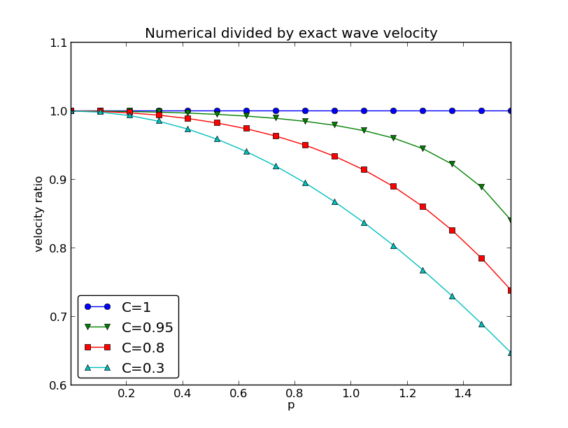
The fractional error in the wave velocity for different Courant numbers

Defining

def r(C, p):
    return 2/(C*p)*asin(C*sin(p))

we can plot \(r(C,p)\) as a function of \(p\) for various values of \(C\), see Figure The fractional error in the wave velocity for different Courant numbers. Note that the shortest waves have the most erroneous velocity, and that short waves move more slowly than they should.

With sympy we can also easily make a Taylor series expansion in the discretization parameter \(p\):

>>> C, p = symbols('C p')
>>> rs = r(C, p).series(p, 0, 7)
>>> print rs
1 - p**2/6 + p**4/120 - p**6/5040 + C**2*p**2/6 -
C**2*p**4/12 + 13*C**2*p**6/720 + 3*C**4*p**4/40 -
C**4*p**6/16 + 5*C**6*p**6/112 + O(p**7)
>>> # Factorize each term and drop the remainder O(...) term
>>> rs_factored = [factor(term) for term in rs.lseries(p)]
>>> rs_factored = sum(rs_factored)
>>> print rs_factored
p**6*(C - 1)*(C + 1)*(225*C**4 - 90*C**2 + 1)/5040 +
p**4*(C - 1)*(C + 1)*(3*C - 1)*(3*C + 1)/120 +
p**2*(C - 1)*(C + 1)/6 + 1

We see that \(C=1\) makes all the terms in rs_factored vanish, except the last one. Since we already know that the numerical solution is exact for \(C=1\), the remaining terms in the Taylor series expansion will also contain factors of \(C-1\) and cancel for \(C=1\).

From the rs_factored expression above we also see that the leading order terms in the error of this series expansion are

\[\frac{1}{6}\left(\frac{k\Delta x}{2}\right)^2(C^2-1) = \frac{k^2}{24}\left( c^2\Delta t^2 - \Delta x^2\right),\]

pointing to an error \({\mathcal{O}(\Delta t^2, \Delta x^2)}\), which is compatible with the errors in the difference approximations (\(D_tD_t\) and \(D_xD_x\)).

Extending the analysis to 2D and 3D

The typical analytical solution of a 2D wave equation

\[u_{tt} = c^2(u_{xx} + u_{yy}),\]

is a wave traveling in the direction of \(\boldsymbol{k} = k_x\boldsymbol{i} + k_y\boldsymbol{j}\), where \(\boldsymbol{i}\) and \(\boldsymbol{j}\) are unit vectors in the \(x\) and \(y\) directions, respectively. Such a wave can be expressed by

\[u(x,y,t) = g(k_xx + k_yy - kct)\]

for some twice differentiable function \(g\), or with \(\omega =kc\), \(k=|\boldsymbol{k}|\):

\[u(x,y,t) = g(k_xx + k_yy - \omega t){\thinspace .}\]

We can in particular build a solution by adding complex Fourier components of the form

\[\exp{(i(k_xx + k_yy - \omega t))} {\thinspace .}\]

A discrete 2D wave equation can be written as

(13)\[ \lbrack D_tD_t u = c^2(D_xD_x u + D_yD_y u)\rbrack^n_{q,r} {\thinspace .}\]

This equation admits a Fourier component

(14)\[ u^n_{q,r} = \exp{\left( i(k_x q\Delta x + k_y r\Delta y - \tilde\omega n\Delta t)\right)},\]

as solution. Letting the operators \(D_tD_t\), \(D_xD_x\), and \(D_yD_y\) act on \(u^n_{q,r}\) from (14) transforms (13) to

\[\frac{4}{\Delta t^2}\sin^2\left(\frac{\tilde\omega\Delta t}{2}\right) = c^2 \frac{4}{\Delta x^2}\sin^2\left(\frac{k_x\Delta x}{2}\right) + c^2 \frac{4}{\Delta y^2}\sin^2\left(\frac{k_y\Delta y}{2}\right) {\thinspace .}\]

or

\[\sin^2\left(\frac{\tilde\omega\Delta t}{2}\right) = C_x^2\sin^2 p_x + C_y^2\sin^2 p_y,\]

where we have eliminated the factor 4 and introduced the symbols

\[C_x = \frac{c^2\Delta t^2}{\Delta x^2},\quad C_y = \frac{c^2\Delta t^2}{\Delta y^2}, \quad p_x = \frac{k_x\Delta x}{2},\quad p_y = \frac{k_y\Delta y}{2}{\thinspace .}\]

For a real-valued \(\tilde\omega\) the right-hand side must be less than or equal to unity in absolute value, requiring in general that

(15)\[ C_x^2 + C_y^2 \leq 1 {\thinspace .}\]

This gives the stability criterion, more commonly expressed directly in an inequality for the time step:

(16)\[ \Delta t \leq \frac{1}{c} \left( \frac{1}{\Delta x^2} + \frac{1}{\Delta y^2}\right)^{-{1/2}}\]

A similar, straightforward analysis for the 3D case leads to

\[\Delta t \leq \frac{1}{c}\left( \frac{1}{\Delta x^2} + \frac{1}{\Delta y^2} + \frac{1}{\Delta z^2}\right)^{-{1/2}}\]

In the case of a variable coefficient \(c^2=c^2(\boldsymbol{x})\), we must use the worst-case value

\[\bar c = \sqrt{\max_{\boldsymbol{x}\in\Omega} c^2(\boldsymbol{x})}\]

in the stability criteria. Often, especially in the variable wave velocity case, it is wise to introduce a safety factor \(\beta\in (0,1]\) too:

\[\Delta t \leq \beta \frac{1}{\bar c} \left( \frac{1}{\Delta x^2} + \frac{1}{\Delta y^2} + \frac{1}{\Delta z^2}\right)^{-{1/2}}\]

The exact numerical dispersion relations in 2D and 3D becomes, for constant \(c\),

\[\tilde\omega = \frac{2}{\Delta t}\sin^{-1}\left( \left( C_x^2\sin^2 p_x + C_y^2\sin^ p_y\right)^\frac{1}{2}\right),\]

\[\tilde\omega = \frac{2}{\Delta t}\sin^{-1}\left( \left( C_x^2\sin^2 p_x + C_y^2\sin^ p_y + C_z^2\sin^ p_z\right)^\frac{1}{2}\right){\thinspace .}\]

We can visualize the numerical dispersion error in 2D much like we did in 1D. To this end, we need to reduce the number of parameters in \(\tilde\omega\). The direction of the wave is parameterized by the polar angle \(\theta\), which means that

\[k_x = k\sin\theta,\quad k_y=k\cos\theta{\thinspace .}\]

A simplification is to set \(\Delta x=\Delta y=h\). Then \(C_x=C_y=c\Delta t/h\), which we call \(C\). Also,

\[p_x=\frac{1}{2} kh\cos\theta,\quad p_y=\frac{1}{2} kh\sin\theta{\thinspace .}\]

The numerical frequency \(\tilde\omega\) is now a function of three parameters:

• \(C\) reflecting the number cells a wave is displaced during a time step
• \(kh\) reflecting the number of cells per wave length in space
• \(\theta\) expressing the direction of the wave

We want to visualize the error in the numerical frequency. To avoid having \(\Delta t\) as a free parameter in \(\tilde\omega\), we work with \(\tilde c/c\), because the fraction \(2/\Delta t\) is then rewritten as

\[\frac{2}{kc\Delta t} = \frac{2}{2kc\Delta t h/h} = \frac{1}{Ckh},\]

and

\[\frac{\tilde c}{c} = \frac{1}{Ckh} \sin^{-1}\left(C\left(\sin^2 ({\frac{1}{2}}kh\cos\theta) + \sin^2({\frac{1}{2}}kh\sin\theta) \right)^\frac{1}{2}\right){\thinspace .}\]

We want to visualize this quantity as a function of \(kh\) and \(\theta\) for some values of \(C\leq 1\). It is instructive to make color contour plots of \(1-\tilde c/c\) in polar coordinates with \(\theta\) as the angular coordinate and \(kh\) as the radial coordinate.

The stability criterion (15) becomes \(C\leq C_{\max} = 1/\sqrt{2}\) in the present 2D case with the \(C\) defined above. Let us plot \(1-\tilde c/c\) in polar coordinates for \(C_{\max}, 0.9C_{\max}, 0.5C_{\max}, 0.2C_{\max}\). The program below does the somewhat tricky work in Matplotlib, and the result appears in Figure Error in numerical dispersion in 2D. From the figure we clearly see that the maximum \(C\) value gives the best results, and that waves whose propagation direction makes an angle of 45 degrees with an axis are the most accurate.

def dispersion_relation_2D(kh, theta, C):
    arg = C*sqrt(sin(0.5*kh*cos(theta))**2 +
                 sin(0.5*kh*sin(theta))**2)
    c_frac = 2./(C*kh)*arcsin(arg)

    return c_frac

from numpy import exp, sin, cos, linspace, \
     pi, meshgrid, arcsin, sqrt
r = kh = linspace(0.001, pi, 101)
theta = linspace(0, 2*pi, 51)
r, theta = meshgrid(r, theta)

# Make 2x2 filled contour plots for 4 values of C
import matplotlib.pyplot as plt
C_max = 1/sqrt(2)
C = [[C_max, 0.9*C_max], [0.5*C_max, 0.2*C_max]]
fix, axes = plt.subplots(2, 2, subplot_kw=dict(polar=True))
for row in range(2):
    for column in range(2):
        error = 1 - dispersion_relation_2D(
            kh, theta, C[row][column])
        print error.min(), error.max()
        cax = axes[row][column].contourf(
            theta, r, error, 50, vmin=0, vmax=0.36)
        axes[row][column].set_xticks([])
        axes[row][column].set_yticks([])

# Add colorbar to the last plot
cbar = plt.colorbar(cax)
cbar.ax.set_ylabel('error in wave velocity')
plt.savefig('disprel2D.png')
plt.savefig('disprel2D.pdf')
plt.show()

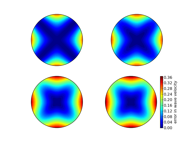
Error in numerical dispersion in 2D